Evolutionary algorithms for scheduling operations
KHMELEVA, ElenaAvailable from Sheffield Hallam University Research Archive (SHURA) at:
http://shura.shu.ac.uk/15608/
This document is the author deposited version. You are advised to consult the publisher's version if you wish to cite from it.
Published version
KHMELEVA, Elena (2016). Evolutionary algorithms for scheduling operations. Doctoral, Sheffield Hallam University.
Copyright and re-use policy
See http://shura.shu.ac.uk/information.html
Sheffield Hallam University Research Archive
Evolutionary Algorithms for
Scheduling Operations
Elena Khmeleva
A thesis submitted to Sheffield Hallam University
for the degree of
DOCTOR OF PHILOSOPHY
i
Abstract
While business process automation is proliferating through industries and
processes, operations such as job and crew scheduling are still performed
manually in the majority of workplaces. The linear programming techniques are
not capable of automated production of a job or crew schedule within a
reasonable computation time due to the massive sizes of real-life scheduling
problems. For this reason, AI solutions are becoming increasingly popular,
specifically Evolutionary Algorithms (EAs).
However, there are three key limitations of previous studies researching
application of EAs for the solution of the scheduling problems. First of all, there
is no justification for the selection of a particular genetic operator and conclusion
about their effectiveness. Secondly, the practical efficiency of such algorithms is
unknown due to the lack of comparison with manually produced schedules.
Finally, the implications of real-life implementation of the algorithm are rarely
considered.
This research aims at addressing all three limitations. Collaborations with
DB-Schenker, the rail freight carrier, and Garnett-Dickinson, the printing company,
have been established. Multi-disciplinary research methods including document
analysis, focus group evaluations, and interviews with managers from different
levels have been carried out. A standard EA has been enhanced with developed
within research intelligent operators to efficiently solve the problems.
Assessment of the developed algorithm in the context of real life crew scheduling
problem showed that the automated schedule outperformed the manual one by
3.7% in terms of its operating efficiency. In addition, the automatically produced
schedule required less staff to complete all the jobs and might provide an
additional revenue opportunity of £500 000.
The research has also revealed a positive attitude expressed by the operational
and IT managers towards the developed system. Investment analysis
demonstrated a 41% return rate on investment in the automated scheduling
system, while the strategic analysis suggests that this system can enable
attainment of strategic priorities. The end users of the system, on the other hand,
ii
Acknowledgements
I would like to sincerely thank my supervisors Professor Adrian Hopgood, Dr
Malihe Shahidan, Mr Lucian Tipi and Dr Jonathan Gorst for their guidance and
support. Owning to their extremely helpful advice, necessary resources and
encouragement, I was able to conduct a very challenging and interesting
research project, achieve good results, participate in various competitions and
win various awards.
I would also like to express my gratitude to DB-Schenker and Garnett-Dickinson
for their participation in my research. My research would not be possible without
the data provided by the aforementioned companies. I also appreciate the time
all the participants from both companies spent explaining to me their extremely
complex processes, sharing their professional knowledge and providing
evaluations throughout the development of my research algorithm.
I would like to say a special thanks to Adrian Hopgood for an opportunity to attend
external conferences and events, which enabled me to present my research and
expand my knowledge outside my immediate research areas.
I am grateful to Mr Lucian Tipi, Malihe Shahidan, Jonathan Gorst and Jamie
Rundle for introducing me to teaching, which allowed me to share my knowledge
with students.
Finally, I would also like to thank Sheffield Business School for partly sponsoring
1
Table of contents
Abstract ... i
Acknowledgements ... ii
Table of contents ... 1
Chapter 1. Introduction ... 15
1.1 Planning and scheduling technologies ... 16
1.2 Research question and objectives ... 18
1.3 DB-Schenker ... 19
1.4 Garnett-Dickinson ... 20
1.5 Justification of research collaborators ... 20
1.6 Research contributions ... 21
1.7 Publications resulting from this thesis ... 22
1.8 Organisation of the thesis ... 22
1.9 Chapter summary ... 25
Chapter 2. Overview of optimisation methods ... 26
2.1 Introduction ... 26
2.2 Heuristic methods ... 26
2.2.1 GRASP (greedy randomized adaptive search procedure) ... 27
2.3 Metaheuristic methods ... 27
2.3.1 Simulated annealing ... 29
2.3.2 Tabu search ... 31
2.3.3 Ant colony optimisation ... 32
2.3.4 Genetic algorithm ... 33
2.4 Hyper-heuristic and multi-purpose algorithms ... 34
2.4.1 Reconfigurable schedulers ... 34
2.4.2 Hyper-heuristics ... 35
2.5 Algorithm comparison and analysis ... 37
2.6 Justification of the selected technique ... 40
2.7 Detailed analysis of EAs ... 40
2.7.1 Chromosome representation ... 41
2.7.2 Population ... 42
2
2.7.4 Selection ... 43
2.7.5 Elitism ... 44
2.7.6 Schemata theorem ... 44
2.7.7 Crossover ... 46
2.7.8 Mutation ... 51
2.7.9 EA parameters ... 52
2.7.10 Local search ... 52
2.8 Conclusion ... 53
Chapter 3. Multi-disciplinary research methods for real life problems ... 54
3.1 Introduction ... 54
3.2 Overview of research structure ... 54
3.3 Data collection methods ... 56
3.3.1 Document analysis ... 57
3.3.2 Interview ... 58
3.3.3 Observation ... 59
3.3.4 Problem modelling ... 60
3.3.5 Prototyping ... 61
3.4 Algorithm parameter selection ... 62
3.5 Algorithm evaluation and business impact assessment ... 63
3.5.1 Cost-benefit analysis ... 63
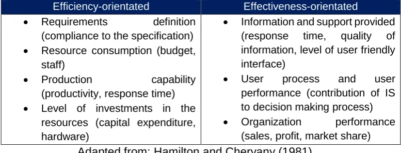
3.5.2 Metrics ... 65
3.5.3 Operational level ... 66
3.5.4 Strategic Level ... 68
3.5.5 Investment Evaluation ... 69
3.6 Conclusion ... 70
Chapter 4. Job-shop Scheduling Problem in the printing Industry ... 71
4.1 Introduction ... 71
4.2 Printing industry overview ... 71
4.3 Job shop scheduling operations in the printing industry ... 72
4.4 Estimator ... 72
4.5 Planner ... 73
4.6 Job-floor ... 73
4.7 Mailing ... 74
4.8 Importance of the scheduling operations ... 74
3
4.10 Performance indicators ... 75
4.11 Problem modelling and formulation ... 75
4.12 Formal definition of the job shop scheduling problem ... 76
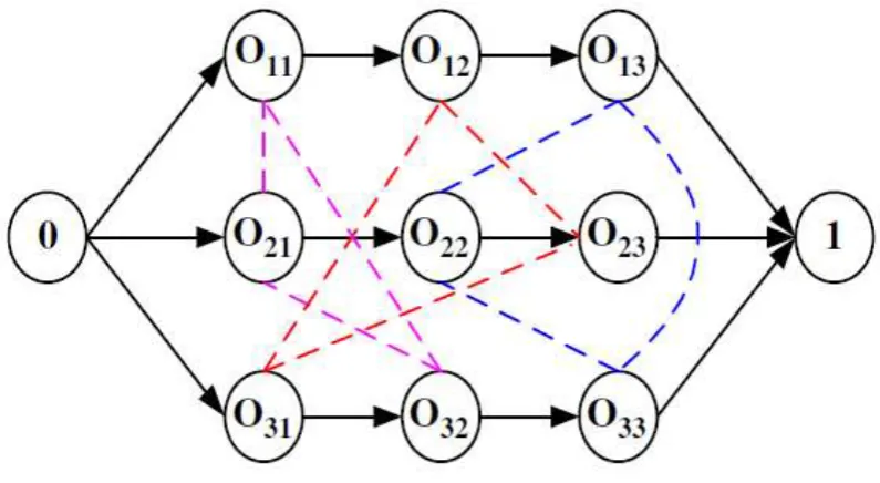
4.13 Disjunctive graph representation classic JSSP ... 77
4.14 Conclusion ... 78
Chapter 5. Approaches to Job Shop Scheduling Problem ... 79
5.1 Introduction ... 79
5.2 Dispatching Rules ... 79
5.3 Giffler and Thomson algorithm ... 80
5.4 Branch and bound (B&B) ... 81
5.5 Metaheuristic algorithms ... 82
5.6 Evolutionary algorithms ... 83
5.6.1 Chromosome representations ... 83
5.6.2 Population management ... 90
5.6.3 Crossover ... 91
5.6.4 Mutation ... 93
5.6.5 Hybrids and local search strategies ... 95
5.6.6 Local neighbourhood search ... 95
5.7 Simulated Annealing (SA) and Tabu Search (TS) ... 95
5.8 Limitations and gaps in the literature ... 97
5.9 Conclusion ... 97
Chapter 6. Crew Scheduling Problem in the rail-freight industry ... 98
6.1 Introduction ... 98
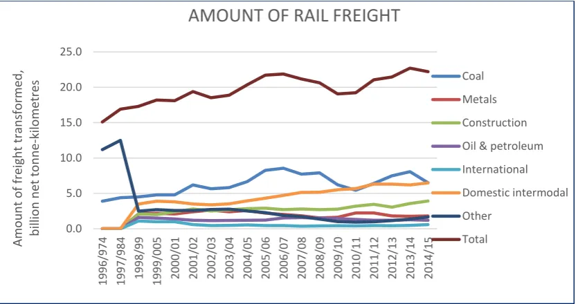
6.2 Role of rail freight in the economy ... 98
6.3 Rail-freight industry overview ... 99
6.4 Planning operations in the rail scheduling ... 101
6.5 Crew Scheduling Problem ... 102
6.5.1 Contractual terms ... 103
6.5.2 Crew scheduling processes ... 103
6.5.3 Operational objectives ... 104
6.5.4 Labour rules ... 104
6.6 Complexity and size of the problem ... 105
6.7 Importance of effective crew scheduling systems ... 105
6.8 Mathematical formulation of the CSP ... 106
4
Chapter 7. Approaches to Crew Scheduling Problem ... 110
7.1 Introduction ... 110
7.2 General approach for the solution of CSP with exact methods ... 110
7.2.1 Column generation ... 113
7.2.2 Master problem ... 114
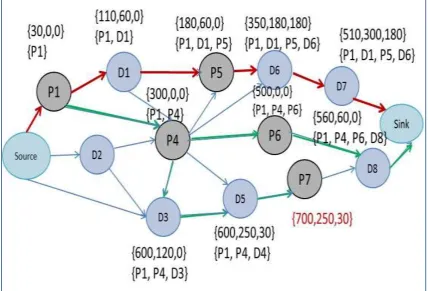
7.2.3 Diagram Generation ... 116
7.2.4 Diagram generation with pricing problem ... 118
7.2.5 Label-setting algorithm for diagram generation ... 119
7.3 Diagram set selection ... 121
7.3.1 Branch-and-bound ... 122
7.3.2 Branching strategies ... 124
7.3.3 Branch-and-price and Branch-and-Cut ... 125
7.4 Metaheuristic methods ... 127
7.4.1 Simulated Annealing ... 127
7.4.2 Ant colony optimisation ... 129
7.4.3 EA algorithm ... 129
7.4.4 EA for diagram generation ... 129
7.4.5 EA for optimization ... 129
7.4.6 Chromosome representations ... 130
7.4.7 Selection ... 133
7.4.8 Crossover ... 134
7.4.9 Mutation ... 135
7.4.10 Constraint handling and infeasibility ... 136
7.4.11 Repair operators ... 136
7.4.12 EA enhancement ... 138
7.5 Other metaheuristic approaches ... 139
7.6 Conclusion ... 140
Chapter 8. Evolutionary algorithm design ... 144
8.1 Introduction ... 144
8.2 Key principles of EA design ... 144
8.3 Analysis of the CSP and JSSS ... 145
8.4 Proposed EA test framework ... 146
8.4.1 Crossover operators ... 147
8.4.2 Mutation ... 148
5
8.4.4 Selection ... 150
8.4.5 Replacement ... 151
8.4.6 Data Instances ... 151
8.4.7 Adaptation to the CSP ... 152
8.4.8 Decoding procedure ... 152
8.4.9 Fitness Function ... 154
8.4.10 Problem-specific crossover for CSP ... 155
8.4.11 Problem-specific mutation for CSP ... 155
8.5 Adaptation to the Job-Shop Scheduling Problem ... 156
8.5.1 Chromosome representation and decoding procedure ... 156
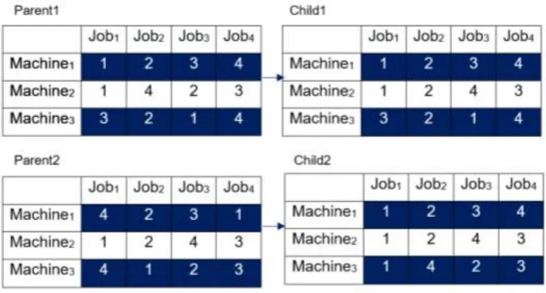
8.5.2 Problem-specific crossover operator ... 158
8.5.3 Problem-specific mutation operator ... 159
8.6 Conclusion ... 160
Chapter 9. Comparison of evolutionary operators and strategies: experimental results ... 162
9.1 Introduction ... 162
9.2 Crew Scheduling Problem ... 162
9.2.1 Single crossover and mutation experiments ... 162
9.2.2 Crossover performance... 163
9.2.3 Mutation performance ... 165
9.2.4 Crossover and mutation ... 168
9.2.5 Multiple operators ... 172
9.2.6 First strategy ... 172
9.2.7 Third strategy ... 174
9.2.8 Comparison of all strategies ... 178
9.4 Classic Job-Shop Scheduling Problem ... 182
9.4.1 Crossover performance... 182
9.4.2 Mutation performance ... 183
9.4.3 Crossover and mutation ... 185
9.4.4 First strategy ... 188
9.4.5 Third strategy ... 190
9.4.6 Comparison of all strategies ... 194
9.5 Comparison and result discussion ... 197
9.5.1 Single operator performance ... 197
6
9.6 Conclusions ... 202
Chapter 10. EA Adaptation to the CSP problem ... 204
10.1 Introduction ... 204
10.2 Chromosome representation supporting evolution of drivers' role ... 205
10.2.1 Genetic operators and their effectiveness in the driver evolution 206 10.3 Nearest Driver ... 208
10.3.1 Fitness function adaptation for the Nearest Driver algorithm ... 208
10.3.2 Nearest Driver results ... 209
10.4 Comparison of all successful techniques ... 210
10.5 Conclusion ... 222
Chapter 11. Implication of the research for an organisation ... 223
11.1 Introduction ... 223
11.2 Overview of the adaptation process ... 223
11.3 Data preparation ... 224
11.3.1 Passenger trains and taxis ... 224
11.3.2 Company trains ... 226
11.3.3 Drivers... 229
11.3.4 EA modification ... 229
11.3.5 Solution construction ... 231
11.3.6 Proof of concept design ... 231
11.4 Optimisation of the real-data set with Nearest Driver EA ... 233
11.5 Cost-benefit analysis of the generalizable algorithm ... 234
11.5.1 Cost ... 234
11.5.2 Benefit ... 235
11.5.3 Cost-benefit analysis ... 237
11.6 Results evaluation and discussion ... 238
11.6.1 Diagram sample evaluation ... 240
11.6.2 Overall impression ... 242
11.6.3 IT perspective ... 246
11.6.4 HR perspective ... 246
11.7 Investment evaluation ... 247
11.7.1 Cost ... 248
11.7.2 Benefits ... 249
7
11.8 Operational perspective ... 251
11.9 Strategy ... 252
11.9.1 Description of DB-Schenker’s Strategy ... 252
11.9.2 Alignment of the Automatic Scheduling System with the strategic goals 254 11.10 Conclusion ... 256
Chapter 12. Conclusions and future research directions ... 258
12.1 Introduction ... 258
12.2 The limitations of the algorithm experiments ... 261
12.3 The limitation of business evaluation ... 261
12.4 Future research direction ... 262
12.5 Final remarks ... 264
Bibliography ... 266
Appendix 1. Focus group discussion ... 290
Appendix 2. Printing Job Schedule ... 291
Appendix 3. Printing job floor ... 292
Appendix 4. Traction types ... 293
Appendix 5. Data Instances for JSSP ... 294
Appendix 6. CSP Crossover and mutation ... 297
Appendix 7. JSSP: Crossover and mutation JSSP ... 303
Appendix 8. Driver Evolution ... 309
Appendix 9. Nearest Driver ... 310
Appendix 10. Process of evolution of real data schedule ... 311
Appendix 11. Evaluated diagrams ... 314
8
List of figures
Figure 1 Worldwide annual supply of industrial robots ... 15
Figure 2 Hyper-heuristics chromosome representation ... 36
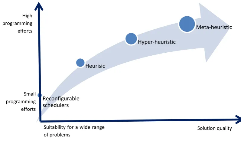
Figure 3 Generalizability of the algorithms level of programming efforts ... 38
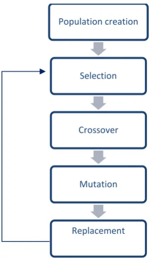
Figure 4 Flow chart of GA ... 41
Figure 5 Schemata instance ... 45
Figure 6 One-point crossover ... 47
Figure 7 Two-point crossover... 47
Figure 8 Uniform crossover ... 48
Figure 9 Partially mapped crossover (PMX) ... 48
Figure 10 Position-based crossover ... 49
Figure 11 Order crossover ... 49
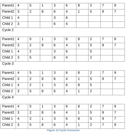
Figure 12 Cycle Crossover ... 50
Figure 13 Insert mutation ... 51
Figure 14 Swap mutation ... 51
Figure 15 Inversion mutation ... 51
Figure 16 Scramble mutation ... 52
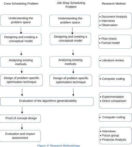
Figure 17 Research Methodology ... 56
Figure 18 Key business operations in the printing industry ... 72
Figure 19 Disjunctive graph representation of JSSP ... 77
Figure 20 Methods for the solution of JSSP ... 82
Figure 21 Job-based chromosome representation ... 84
Figure 22 Operation-based chromosome representation ... 85
Figure 23 Job-pair relationship based chromosome representation ... 86
Figure 24 Completion time-based chromosome representation ... 86
Figure 25 Random-keys chromosome representation ... 87
Figure 26 Random key chromosome representation with delay times ... 87
Figure 27 Preference list-based chromosome representation ... 88
Figure 28 Disjunctive based chromosome representation ... 90
Figure 29 Modified Precedence Operation Crossover ... 92
Figure 30 Subsequence exchange crossover ... 93
Figure 31 Job-based ordered crossover ... 93
Figure 32 Neighbourhood mutation ... 94
Figure 33 Demand for rail freight transportation by commodity 1996-2014 .... 100
Figure 34. The main operations of the railways freight carrier ... 102
Figure 35 Trains in the timetable... 111
Figure 36 Diagrams ... 111
Figure 37 Connection graph ... 117
Figure 38 Time space network ... 117
Figure 39 Label-setting algorithm ... 120
Figure 40 Continuous solution ... 122
Figure 41 Linear program with constraints ... 126
9
Figure 43 Binary Chromosome representation ... 131
Figure 44 Integer Chromosome representation ... 131
Figure 45 Adaptive chromosome representation ... 132
Figure 46 Expressed and Unexpressed genes ... 133
Figure 47 Graph-based chromosome representation ... 133
Figure 48 Heuristic used in the literature for CSP ... 140
Figure 49 EA for CSP and JSSP test framework ... 147
Figure 50 Chromosome representation and decoding logic ... 153
Figure 51 Intelligent crossover ... 155
Figure 52 Intelligent Mutation ... 156
Figure 53 Comparison of decoding procedures for JSSP ... 158
Figure 54 Problem-Specific Crossover for JSSP ... 159
Figure 55 Intelligent Mutation ... 160
Figure 56 Performance of different crossover operators on a small CSP data set ... 163
Figure 57 Performance of different crossover operators on a medium CSP data set ... 163
Figure 58 Performance of different crossover operators on a large CSP data set ... 164
Figure 59 Performance of different mutation operators on the small CSP data set ... 166
Figure 60 Performance of different mutation operators on the medium CSP data set ... 166
Figure 61 Performance of different mutation operators on the large CSP data set ... 166
Figure 62 Example when scramble mutation deteriorates the schedule ... 168
Figure 63 Example when a simple mutation does not change a driver schedule ... 168
Figure 64 Performance of the pair of crossover and mutation on the small data set ... 169
Figure 65 Performance of the pair of crossover and mutation on the medium data set ... 170
Figure 66 Performance of the pair of crossover and mutation on the large data set ... 171
Figure 67 Contribution of each operator in Strategy 1 ... 173
Figure 68 Strategy3: Contribution and utilisation of each crossover operator for CSP ... 176
Figure 69 Contribution and utilisation of each mutation operator for CSP ... 177
Figure 70 Performance of different strategies on a small data set ... 179
Figure 71 Performance of different strategies on a medium data set ... 179
Figure 72 Performance of different strategies on a large data set ... 179
Figure 73 Final results produced by each strategy on a small data set ... 180
Figure 74 Final results produced by each strategy on a medium data set ... 180
Figure 75 Final results produced by each strategy on a medium data set ... 181
10
Figure 77 Performance of crossovers on a medium JSSP data set ... 182
Figure 78 Performance of crossovers on the large JSSP data set... 183
Figure 79 Performance of different mutation operators on small JSSP data set ... 184
Figure 80 Performance of different mutation operators on medium JSSP data set ... 184
Figure 81 Performance of different mutation operators on large JSSP data set ... 184
Figure 82 Average results achieved by a combination of crossovers and mutation on small JSSP data ... 185
Figure 83 Average results achieved by a combination of crossovers and mutation on medium JSSP data ... 186
Figure 84 Average results achieved by a combination of crossovers and mutation on large JSSP data ... 188
Figure 85 Experimental results of the first strategy applied to JSSP ... 190
Figure 86 Strategy3: Contribution and utilisation of each crossover operator for JSSP ... 192
Figure 87 Contribution and utilisation ratio of mutation operators in the Strategy 3 for JSSP ... 194
Figure 88 Performance of strategies on the small JSSP data set ... 195
Figure 89 Performance of strategies on the medium JSSP data set ... 195
Figure 90 Performance of strategies on the large JSSP data set ... 195
Figure 91 Performance of different strategies on a small JSSP data set ... 196
Figure 92 Performance of different strategies on a medium JSSP data set .... 197
Figure 93 Performance of different strategies on a large JSSP data set ... 197
Figure 94 Impact of LOX crossover on CSP and JSSP ... 199
Figure 95 Impact of PBX crossover on JSSP and CSP ... 200
Figure 96 Example of the population with static drivers ... 205
Figure 97 Example of the population with evolving drivers ... 205
Figure 98 Final results of various driver evolution operators on a small data set ... 207
Figure 99 Final results of various driver evolution operators on a medium data set ... 207
Figure 100 Final results of various driver evolution operators on a large data set ... 207
Figure 101 Comparison of EA configurations: Actual Cost of the Schedule of the small CSP data set ... 211
Figure 102 Comparison of EA configurations: Actual Cost of the Schedule of the medium CSP data set ... 211
Figure 103 Comparison of EA configurations: Actual Cost of the Schedule of the large CSP data set ... 212
Figure 104 Comparison of EA configurations: Number of diagrams on the small CSP data set ... 213
11 Figure 106 Comparison of EA configurations: Number of diagrams on the large
CSP data set ... 214
Figure 107 Comparison of EA configurations: Throttle time on the small CSP data set ... 215
Figure 108 Comparison of EA configurations: Throttle time on the medium data set ... 215
Figure 109 Comparison of EA configurations: Throttle time on the large CSP data set ... 216
Figure 110 Comparison of EA configurations: Average deviation on the medium CSP data set ... 216
Figure 111 Comparison of EA configurations: Average deviation on the large CSP data set ... 217
Figure 112 Comparison of EA configurations: Average deviation for the large CSP data set ... 217
Figure 113 Comparison of EA configurations: Workload distribution among depots for the small CSP data set ... 218
Figure 114 Comparison of EA configurations: Workload distribution among depots for the medium CSP data set ... 218
Figure 115 Comparison of EA configurations: Workload distribution among depots for the large CSP data set ... 219
Figure 116 Comparison of EA configurations: Total Cost of the Schedule of the small CSP data set ... 220
Figure 117 Comparison of EA configurations: Total Cost of the Schedule of the medium CSP data set ... 220
Figure 118 Comparison of EA configurations: Total Cost of the Schedule of the large CSP data set ... 221
Figure 119 Effect of driver Evolution of the Schedule ... 221
Figure 120 The process of testing EA on the real data set ... 224
Figure 121 Example of the data format ... 227
Figure 122 Demonstration of the input data ... 232
Figure 123 Screen shot of the prototype: Selecting EA parameters ... 232
Figure 124 Screen shot of the prototype: evolution process demonstration ... 233
Figure 125 Cost of the schedule and the percentage difference with the most efficient one... 236
Figure 126 Cost difference between the manual schedules and EAs ... 236
Figure 127 Relative benefits among the algorithm ... 237
Figure 128 Relative savings per pound invested ... 238
Figure 129 Example of the diagram produced by the algorithm ... 243
Figure 130 Example of the diagram produced manually ... 243
Figure 131 Key process performance indicators ... 251
Figure 132 Aspects of DB-Schenker’s Strategy (Source: DB-Schenker n/d) .. 254
Figure 133 Focus group discussion plan ... 290
Figure 134 Gantt chart illustrating printing job schedule ... 291
12 Figure 136 Performance of the intelligent crossover with mutations on the small
data set ... 297
Figure 137 Performance of the intelligent crossover with different mutations on the medium data set ... 297
Figure 138 Performance of the intelligent crossover with different mutations on the large data set ... 297
Figure 139 Performance of the PMX crossover with different mutations on the small data set ... 298
Figure 140 Performance of the PMX crossover with different mutations on the medium data set ... 298
Figure 141 Performance of the PMX crossover with different mutations on the medium data set ... 298
Figure 142 Performance of the LOX crossover with different mutations on the small data set ... 299
Figure 143 Performance of the LOX crossover with different mutations on the medium data set ... 299
Figure 144 Performance of the LOX crossover with different mutations on the large data set ... 299
Figure 145 Performance of the PBX crossover with different mutations on the small data set ... 300
Figure 146 Performance of the PBX crossover with different mutations on the medium data set ... 300
Figure 147 Performance of the PBX crossover with different mutations on the large data set ... 300
Figure 148 Performance of the CX crossover with different mutations on the small data set ... 301
Figure 149 Performance of the CX crossover with different mutations on the medium data set ... 301
Figure 150 Performance of the CX crossover with different mutations on the large data set ... 301
Figure 151 Crossover comparison CSP 780 with Intelligent mutation ... 302
Figure 152 Crossover comparison CSP 1260 with intelligent mutation ... 302
Figure 153 Crossover comparison CSP 1980 with intelligent mutation ... 302
Figure 154 Performance of intelligent crossover on small JSSP data set ... 303
Figure 155 Performance of intelligent crossover of medium JSSP data set ... 303
Figure 156 Performance of intelligent crossover on large JSSP data set ... 303
Figure 157 Performance of PMX crossover on small JSSP data set ... 304
Figure 158 Performance of PMX crossover on medium JSSP data set ... 304
Figure 159 Performance of PMX crossover on large JSSP data set... 304
Figure 160 Performance of PBX crossover on a small data set ... 305
Figure 161 Performance of PBX crossover on a medium data set ... 305
Figure 162 Performance of PBX crossover on a medium data set ... 305
Figure 163 Performance of CX crossover on a small data set ... 306
Figure 164 Performance of CX crossover on a medium JSSP data set ... 306
13
Figure 166 Performance of LOX crossover on a small JSSP data set ... 307
Figure 167 Performance of LOX crossover on a medium JSSP data set ... 307
Figure 168 Performance of LOX crossover on a large JSSP data set ... 307
Figure 169 Performance of crossovers on the small size of JSSP... 308
Figure 170 Performance of crossovers on the medium size of JSSP ... 308
Figure 171 Performance of crossovers on the large size of JSSP ... 308
Figure 172 Driver Evolution on a small data set... 309
Figure 173 Driver Evolution on a medium data set ... 309
Figure 174 Driver Evolution on the large data sets ... 309
Figure 175 Nearest Driver evolution process on the small data set ... 310
Figure 176 Nearest Driver evolution process on the medium data set ... 310
Figure 177 Nearest Driver evolution process on the large data set ... 310
Figure 178 Evolution process: Total Cost of the Schedule ... 311
Figure 179 Evolution process: Driver Cost ... 311
Figure 180 Evolution process: Total Cost of Deadheads ... 312
Figure 181 Evolution process: Cost of workload distribution ... 312
Figure 182 Evolution process: Total Cost of the deviation of the shift length .. 313
14
List of tables
Table 1 Advantages and disadvantages of metaheuristic methods ... 28
Table 2 Cooling Schedule ... 30
Table 3 Development time and Generalizability of the algorithms ... 37
Table 4 Comparative analysis of the heuristic and meta-heuristic methods ... 39
Table 5 List of required data ... 58
Table 6. MIS performance measures ... 65
Table 7 Chromosome representation of JSSP ... 83
Table 8 Problem Complexity ... 105
Table 9 Diagram cost ... 112
Table 10 Deadheads ... 112
Table 11 Conceptual comparison of CSP and JSSP ... 145
Table 12 Data sets for CSP experiments ... 151
Table 13 Data sets for the JSSP experiments ... 152
Table 14 Average results of crossover and mutation performance for CSP780 ... 169
Table 15 Average results of crossover and mutation performance for CSP1260 ... 170
Table 16 Average results of crossover and mutation performance for CSP1980 ... 171
Table 17 Average crossover and mutation result for the small size JSSP... 186
Table 18 Average results obtained by crossover and mutation operator on medium JSSP ... 187
Table 19 Average results obtained by crossover and mutation operator on large JSSP ... 188
Table 20 Strategy 3 Parameters for JSSP ... 191
Table 21 The Nearest Driver experimental results ... 210
Table 22 Real life train data set comparison... 228
Table 23 Types and specification of the deadhead transportation ... 230
Table 24 Average cost of EA- produced schedule on the real data ... 234
Table 25 Algorithm development efforts ... 235
Table 26 Algorithm development cost ... 235
Table 27 Comparison of the cost of manually and automatically produced schedules239 Table 28 Automatic Crew Scheduling System Investment Analysis ... 248
Table 29 Labour cost for scheduling system development ... 249
Table 30 Automatic Scheduler alignment with the organisational strategy ... 255
15
Chapter 1.
Introduction
In recent years technology has been developing at an exponential pace
revolutionising business operations and re-shaping customer experience
(Kurzweil 2006). Such products as Google Home and Amazon Echo are taking
control of homes by being able to understand commands in natural language and
remotely operate various appliances and devices (Brandon, 2016). Chatbots like
Amelia can answer standard questions and handle a natural conversation with
customers, while sophisticated algorithms are capable of predicting future
purchases and making personalised product recommendations (Business Wire
2014, Fang, Zhang and Chen 2016, Zhang and Song 2015, Da-Cheng Nie, et al.
2014).
These rapid advancements in AI and their proliferation in day-to-day life are
beginning a new technological era. Researchers and practitioners mark this time
as the fourth industrial revolution or industry 4.0 (Baur and Wee 2015).
According to the Forrester research agency, $2.06 trillion have been invested
globally in software, hardware, and IT services by enterprises and governments
in 2013 (Lunden 2013). The number of supplied industrial robots is increasing
every year. According to the International Federation of Robotics (2015), it
reached 229,000 units in 2014 with eighty percent of executives believing that AI improves workers’ performance and creates jobs (Narrative Science 2015).
Figure 1 Worldwide annual supply of industrial robots
16
Von Rosing and Polovina (2015, p.196) state that “Business processes are the
heart of an organization and the support of the business processes by application systems is central to each organization”. Moreover, in today’s rapidly changing
business environment and increasing volumes of available information, it is
impossible to make an adequate analysis and to take a rational decision without
the aid of an information system. Baltzan (2009, p.60) describes this challenge as “Highly complex decisions involving far more information than the human brain can comprehend must be made in increasingly shorter time frames".
However, to date, not all companies have a powerful information system, which
can assist them with data analysis and decision making. From eighty to
eighty-five percent of information remain uncaptured by some of enterprise applications (Polovina 2013). Mckinsey’s global survey of 807 executives shows that a large
number of respondents expressed dissatisfaction with their current IT solutions.
Moreover, respondents claim that their IT is becoming less effective in helping
them achieve strategic objectives (Khan and Sikes 2014).
1.1
Planning and scheduling technologies
An example of such analytical decisions are planning and scheduling operations.
Planning and scheduling processes are the backbone operations in many
organisations. Effective planning and scheduling enable successful assignment
of limited resources to required jobs and often determine the overall cost for the
project. As the number of regulations and tasks in the value chains of medium
and large businesses increases, building an optimal manual schedule becomes
an extremely hard, if not impossible task.
While the automotive and electronics industries are relatively automated (Figure
1), the railway and printing industries are lagging behind. For example, Withall,
et al. (2011) and Clarke, et al. (2010) observe that such decisions as platform
allocation and rolling stock scheduling are made by humans with very limited
assistance from information systems. This research will also show that the
complex train driver scheduling decisions in the rail-freight industry and
job-scheduling decisions in the printing industry are performed manually as well.
Various existing commercial scheduling software such as ShiftPlanning, Appointy
17 scheduling problems, so the assignment decision itself is still made by humans
(WhenToWork 2016, Appointy 2016, ShiftPlanning 2016) .
There are two key questions which one needs to answer when designing a
scheduling system. First of all, what algorithm can be incorporated to produce
and optimise the schedule? And, secondly, would it be possible to apply the same
algorithm for different problems in order to achieve economies of scale and to
reduce the development cost?
Traditionally scheduling problems have been solved with linear programming
techniques. Linear programmes were formulated during the Second World War
by Kantorovich and in 1946-1947 Dantzing proposed a Simplex method for its
solution (Wood 1965, Dantzing and Wolfe 1974). Although these methods
provide an optimal solution, they are becoming less and less practical as their
computation time grows exponentially with the increase in the size of the data.
Onwubolu and Babu (200 p.1) state that “The days when researcher emphasised
using deterministic search techniques to find optimal solutions are gone”.
A new generation of algorithms, metaheuristic algorithms, emerged in the
1960s-1970s, which are now becoming increasingly popular (Gogna and Tayal 2013,
Kincaid 2008, Gendreau and Potvin 2005, Blum and Roli 2003). By mimicking
various natural processes, they are able to tackle large volumes of data and arrive
at a sub-optimal solution within an acceptable time frame. For example,
Evolutionary Algorithms (EAs) are a class of metaheuristic algorithms, which
replicate biological evolution and are guided by the Darwinian principle of “the
fittest survives”.
One of the algorithms belonging to this class is the Genetic Algorithm (GA)
developed by John Henry Holland in 1975 (Holland 1975). Unlike other EAs, a
GA uses binary vectors in order to encode the solution. However, similar to many
EAs, a GA is "an artificial intelligence system that mimics the evolutionary,
survival-of-the-fittest process to generate increasingly better solutions to a problem. A GA essentially is an optimizing system: it finds a combination of inputs that gives the best outputs" (Baltzan 2015 p.62). He further states that a GA is best suited to decision making environments in which, thousands, or perhaps
millions, of solutions are possible. This is because it can “find and evaluate
18 Examples of such environments and problems can include the driver scheduling
problem in the rail-freight industry or job-shop scheduling problems in the printing
industry.
Several studies such as Azadeh et al. (2013), Shen et al. (2013), Zeren and Ozkol
(2012), Ozdemir and Mohan (2001) and Levine (1996) have proposed EAs for
the solution of crew scheduling problems. Spanos et al. (2014), Zhang, Gao and
Li (2013), Dong Hui (2012), Meeran and Morshed (2012), Qing-dao-er-ji and
Wang (2012, Yang et al. (2012) and Jia et al. (2011) have developed the
algorithms for the solution of job scheduling problems.
However, despite the popularity of EAs in operations research communities,
there are four areas which are under-researched. These gaps are presented
below.
1. Most of the EAs have been devised to tackle a specific problem. Minimal
research has been conducted regarding applicability of those algorithms
across different domains. Moreover, none of the studies investigated the
benefits and risks of application of the generalizable algorithm in real life.
2. There is no conclusion amongst researchers regarding the efficiency of
genetic operators across different domains.
3. The majority of the developed algorithms have not been tested on real
life sets of data and their practicability is not fully known.
4. There is a lack of knowledge of what impact these algorithms would have
on a broader business performance if they were built in to real
information systems.
This research approaches the problem in a different way. First of all, it works with
real business problems rather than their simplified models. Secondly, it tests the
effectiveness of standard genetic operations across two conceptually different
problems. Finally, it examines the implications of potential utilisation of the
devised algorithm in a real business environment.
1.2
Research question and objectives
The key objective of this research is getting an insight into EA capabilities for the
19 two significantly different formulations of scheduling problems in different
industries. Its potential impact on immediate and long term business performance
will be studied. Given that, the research question and objectives are proposed
below.
RESEARCH QUESTION: Can an EA improve scheduling processes in different real-life situations?
RESEARCH OBJECTIVES:
1. To understand the complexity of scheduling operations in real life.
2. To investigate the performance of standard EA operators against
each other.
3. To develop and evaluate problem-specific operators in the context
of the Crew Scheduling Problem (CSP) and the Job Shop
Scheduling Problem (JSSP).
4. To understand the limitations and challenges in the design of a
generalizable algorithm for different domains.
5. To assess the impact of the automatic crew scheduling system on
the operational and strategic performance in a real distribution
organisation.
In order to achieve the above-mentioned objectives, collaborations with two
companies where scheduling operations play a crucial role have been
established. The companies are briefly introduced below, but their operations are
considered in greater detail in Chapter 4 and Chapter 6.
1.3
DB-Schenker
DB-Schenker is the largest freight rail operator in the UK (DB-Schenker 2014).
Currently DB-Schenker accounts for 39 depots, 1240 drivers and operates 550
trains across the country on a single day. The company transports a wide range
of commodities: from coal and chemicals to consumer goods. One of the main
challenges the company experiences is the efficient utilisation of train drivers
(DB-Schenker Head of HR interviewed on 07/11/2012, DB-Schenker Head of
Finance interviewed on 07/11/2012). The problem becomes very complicated in
20 hours, a fixed-hour annual contract with drivers, railway regulations and demand
uncertainty.
Preliminary research has found that the current information system (IS) is only
able to provide summative historical reports for the team of decision makers. All
processes, in particular complex scheduling and rostering operations, are
executed manually. IS has only a controlling function on these operations and
gives a warning message if the created operation cannot be performed. There is
a need of an optimisation engine for IS, which would automatically analyse a large
amount of data and suggest an effective way of assignment of the train drivers to
the train trips.
1.4
Garnett-Dickinson
Garnett-Dickinson is the second collaborator. This company offers various types
of publications ranging from newspapers and catalogues to high quality
magazines. The volume reaches hundreds of thousands of magazines, millions
of catalogues and brochures a year (Garnett-Dickinson 2012).
Each publication (job) consists of several operations (i.e. printing, folding,
stitching). The task is to assign these operations to the relevant machines in the
sequence which reduces the completion time and does not violate operational
constraints (deadlines, relevance of machines). The effective scheduling
processes can reduce the lead time and fully utilise the capacity
(Garnett-Dickinson Chief Executive interviewed on 16/10/2012, Garnett-(Garnett-Dickinson
Managing Director interviewed on 16/10/2012).
To date, the computer software enables only graphical representation of the
job-shop using "drag & drop" technology; however, all the assigning decisions sit on
the scheduler (Garnett Dickinson Operations Manager interviewed on
20/10/2012) . That makes the company highly dependent on the planners as well
as on their expertise and experience.
1.5
Justification of research collaborators
These companies were chosen for the following reasons:
1. Scheduling operations take a central place in their operational
21 2. They do not have an automated scheduling system, so it would be
possible to carry out an evaluation of how the companies can
leverage the IS solutions based on EAs.
3. The large size of trips, depots, crew, and printing jobs is sufficient
to build a credible model and to make generalisations.
4. The companies are interested in the research and agree to
cooperate
5. They have granted access to documentation, data and permission
to interview members of staff to obtain the required information.
6. The scale of operations and operational conditions are extremely
different. Testing the same algorithm on such diverse problems
would provide reasonably accurate information with regard to its
universal applicability and generalizability.
7. The head offices of both companies are located in South Yorkshire.
This offers an opportunity to make regular visits in order to collect
a sufficient level of information.
Elaborating on the sixth point, it is necessary to highlight the considerable
difference between the problems. The first problem deals with the allocation of
the workforce whereas the second deals with the allocation of jobs, thus both
have very different scheduling rules and constraints (Pinedo 2009). Moreover,
the amount of jobs which need to be allocated to machines in the second problem
are significantly lower than the number of train trips in the first problem. As the
first problem presents a greater optimisation challenge, this will be the focal
example in the thesis.
1.6
Research contributions
This study has made six major academic and practical contributions.
1. The performance of standard genetic operators for two significantly
different scheduling problems has been investigated and the most efficient
operators have been identified.
2. Novel intelligent genetic operators which allow a practical solution to be
found more quickly than conventional operators, while still satisfying all the
22 3. A comprehensive evaluation framework encompassing operational and
strategic factors has been developed and applied.
4. The possibility and associated risk of using the same algorithm to reduce
the software development costs have been examined.
5. The suitability of an EA for real life scheduling operations has been
examined and the operational and economic effect on overall organisation
performance has been assessed.
6. A complex research methodology has been designed for combining
document analysis, interviews, focus groups, and computational
experiments, in order to achieve the above contributions.
1.7
Publications resulting from this thesis
In addition to the aforementioned contributions, the author has produced a
conference paper, which has won the Best Refereed Paper Written by a Student
award in the application stream at 34th Annual International Conference of BCS
Charted Institute for IT in Specialist Group on Artificial Intelligence:
Khmeleva, E., Hopgood, A.A., Tipi, L. and Shahidan, M.
"Rail-Freight Crew Scheduling with a Genetic Algorithm"
Proc. AI-2014, Research and Development in Intelligent Systems XXXI,
M.Bramer and M.Petridis (eds.), Springer, December 2014.
The full text of the publication and the awarded certificate are presented in
Appendix 12.
1.8
Organisation of the thesis
Broadly the structure of the thesis can be divided into three parts. The first part
concerns the design of an appropriate methodology for the research. The second
part provides an insight into real life scheduling operations and devises a model
describing the processes. Finally, the third part deals with the design of the
effective EA and assesses its applicability in a real business environment. The
23 Chapter 1
Introduction
This chapter introduces the research question
and research objectives. It also provides an
overview of the organisations participating in
this research and their scheduling operations.
Chapter 2
Overview of optimisation
methods
The key objective of the chapter is to select and
justify the algorithm which will be incorporated
into the automatic scheduler. In order to
accomplish this, several algorithms will be
critically reviewed and discussed.
Chapter 3
Multi-disciplinary methods for
real life problems
The aim of this chapter is to design an
appropriate methodology which would enable
the capture of complex real life processes as
well as supporting the development of the EA
and its evaluation in real life settings.
Chapter 4
Job-shop scheduling in the
printing industry
This chapter presents the context of job-shop
scheduling in the printing industry and
identifies the challenges that schedulers face
when assigning jobs to printing presses. The
output of this chapter is the model describing
the job shop scheduling process.
Chapter 5
Approaches to job-shop
scheduling problem
This chapter discusses the approaches
developed in the literature for the solution of
job-shop scheduling problems and analyses
their advantages and disadvantages.
Chapter 6
Crew scheduling problems in
the rail-freight industry
This chapter outlines scheduling and planning
operations in the rail-freight transportation
industry. It focuses on the driver scheduling
problems and related health and safety
24 must be taken into account when constructing
a driver working plan.
Chapter 7
Approaches to crew
scheduling problems
This chapter reviews existing approaches to
the solution of crew scheduling problems and
analyses their effectiveness in relation to
real-life scheduling operations.
Chapter 8 EA design
This chapter sets the main principles for
effective EA design and proposes two novel
operators specifically developed in this
research to solve crew scheduling and
job-shop scheduling problems
Chapter 9
Comparison of evolutionary
operators and strategies:
experimental results
This chapter experimentally compares
traditional genetic operators and intelligent
operators devised within this research. It also
empirically validates the joint application of
multiple genetic operators within the same
algorithm and compares the results obtained
for CSP and JSSP.
Chapter 10
Adaptation of the EA to the
CSP problem
This chapter establishes the limitations of the
application of the same algorithm for
conceptually different problems. It enhances
the complexity of the chromosome
representation for CSP to drive the efficiency
of the algorithm. After examination and tests of
various decoding procedures, it selects the
configuration of the algorithm which provides
the most cost-efficient schedule to be applied
25 Chapter 11
Implication of the research
for an organisation
Discusses the adaptation of real life data and
EA objective function to real life CSP. It then
reports the results of the expert evaluation of
the EA produced schedule and analyses the
results. The analysis considers the quality and
practicability of the schedule, the impact on
operational performance and the alignment
with organisation strategy.
Chapter 12
Conclusions and future
research directions
Provides an overall summary of the conducted
research and obtained results. It also outlines
some of the research limitations and suggests
future research directions.
1.9
Chapter summary
This chapter has demonstrated that despite significant technological progression
and increased supply of industrial robots in recent years, complex planning and
scheduling operations are still performed manually. The traditional linear
programming algorithms struggle to handle a large of amount of data and are
becoming replaced by various AI optimisation algorithms. However, the way the
companies in the rail-freight industry can leverage AI based on automated
planning technologies and their impact on their performance is a significantly
under-researched area. The main research question of this study is to devise a
proof of concept of such software and conduct a detailed assessment of its
effectiveness in a real organisation.
The next chapter introduces and closely examines metaheuristic algorithms,
which can be applied to assist companies in solving their crew and job-shop
26
Chapter 2.
Overview of optimisation
methods
2.1
Introduction
The purpose of this chapter is to identify the technique, which can be incorporated
into CSP and JSSP automatic schedule builders. In order to accomplish this,
several optimisation methods for the solution of combinatorial problems will be
reviewed. Their general logic as well as strengths and weaknesses in relation to
the solution of the scheduling problems will be discussed. More importantly,
because this thesis considers their real-life application and business impact, the
development efforts for each algorithm will also be taken into account when
selecting an algorithm. Development efforts will be measured on the basis of two
dimensions: the algorithm complexity (i.e. how long and sophisticated the code
should be) and generalizability (i.e. the possibility to transfer the code to other
problems).
This chapter is focused only on the AI algorithms and does not present exact
techniques. This is because the majority of real-life optimisation problems have
an immense number of constraints and variables and belong to the class of
NP-hard combinatorial problems (Hart, Ross and Nelson (1998), Gogna and Tayal
(2013)). The exact methods usually struggle with such a large number of
variables because they are based on techniques which require generation of all
possible combinations. Since it is almost impossible to produce and evaluate all
possible solutions for NP-hard problems, they have been rejected due to their
impracticability for this research.
2.2
Heuristic methods
Reeves (1993,p.6) provides a definition of heuristic methods.
Definition 1
27
optimality, or even in many cases to state how close to optimality a particular feasible solution is”.
Unlike exact integer programming (IP) techniques, heuristic methods exploit the
nature of combinatorial problems rather than their IP formulation (Gendreau and
Potvin 2005). Since they do not rely on objective function derivatives they have
more chances to escape local optimum as well as handle non-continuous
functions and discrete parameters (Haupt 1998). The downside of this is heuristic
methods are usually tailored to a particular problem and have a limited
applicability to other problems. Design of an effective heuristic method requires
substantial knowledge regarding the domain. One of the examples of heuristic
methods is greedy randomised adaptive search procedure (GRASP), which is
described below.
2.2.1
GRASP (greedy randomized adaptive search procedure)
GRASP is a simple heuristic which consists of two operators: constructive
heuristic and local search (Blum et al. 2011). Construction operator assembles a
solution element by element with a certain degree of randomization. After that the
solution is enhanced with a tailored improvement technique. This is a multi-start
method, which means that the described process repeats a certain number of
times. The memory preserves all final solutions and at the final iteration the best
solution is regarded as a final result (Gendreau and Potvin 2005).
GRASP can provide a solution for a relatively short period of time and can be
incorporated into various algorithmic frameworks (Blum et al. 2011). One of the
drawbacks of GRASP is that it does not rely on the history of the previously
obtained solutions in order to direct the search (Gendreau and Potvin 2005, Blum
et al. 2011). Furthermore, the heuristic technique must be specifically designed
for a particular domain, which reduces the level of generalizability of the algorithm
and requires ample knowledge about the problem.
2.3
Metaheuristic methods
Unlike simple heuristic methods, meta-heuristics are less problem-dependent
28
Definition 2
A metaheuristic is "an iterative generation process which guides subordinate heuristics by combining intelligently different concepts for exploring and exploiting the search space, and learning strategies are used to structure information in order to find efficiently near-optimal solutions" (Osman and Laporte 1996, p.1). In general, heuristic techniques are more flexible and adaptable to real-world
situations than exact methods (Gogna and Tayal 2013). Due to having a variety
of tools for productive exploration and exploitation of search space, they are more
likely to reach the global optima of the function than heuristics methods. Moreover,
these techniques, in many cases, allow the algorithm to escape local optimuma.
As to their disadvantages, the tuning and design of a low level heuristic might be
time-consuming.
Despite the fact that meta-heuristics do not guarantee finding the mathematical
optimum, they are highly capable of finding a reasonable solution for a much
shorter period of time than exact methods. This fact makes meta-heuristics highly
attractive for real life applications (Reeves 1993, Gendreau and Potvin 2005,
Gogna and Tayal 2013).
The summary of the benefits and limitations of metaheuristic methods are
displayed in Table 1.
Table 1 Advantages and disadvantages of metaheuristic methods
Advantages Limitations
• More general applicability than heuristic alone
• Find global optima • Deal with local optimums • Reasonable computation time • Find global optima
• Handle complicating constraints
• Do not guarantee finding the optimum solutions
• Not easy to prove efficiency of the algorithm
• Requires a significant amount of time to be developed
• Analysis and selection of the algorithm for a particular problem is a very challenging task
• Requires extensive knowledge about the problem
Adapted from Gogna and Tayal (2013), Gendreau and Potvin (2005)
The majority of metaheuristic methods were inspired by real life processes. For
29 resembles the brain memory; GA is based on biological evolution and Ant Colony Optimisation imitates ants’ behaviour. These methods as well as their
advantages and limitations will be discussed below.
2.3.1
Simulated Annealing
The logic of Simulated Annealing (SA) algorithm is derived from the Metropolis's
algorithm defining annealing process. Annealing is the chemical transformation
occurring in metals when they undergo temperature changes (Reeves 1993).
Usually the metal is first heated at a very high temperature till the point when it
starts to melt. After that, the temperature starts to drop according to a certain
schedule altering the internal energy and making the structure of metal rigid and
fixed. The process is often applied in metallurgy in order to produce materials of
a high quality with a minimum number of defects (Elhaddad 2012).
Application of annealing principles as an optimisation technique was proposed
by Kirkpatrick et al. (1983). In the optimisation context, the energy of the system
is equivalent to objective function, state of the physical system is represented by
solution and temperature is a control parameter regulating exploitation and
exploration phases (Reeves 1993, Gendreau and Potvin 2005, Gogna and Tayal
2013).
The SA algorithm starts from initialisation of the first candidate and selecting a
temperature. At the beginning, the temperature should be set reasonably high
(Gogna and Tayal 2013). Too low temperature might force the algorithm to
converge around a local optimum. However, if the temperature is set too high the
convergence of the algorithm can be relatively slow. At the next step, the
candidate solution, lying in the neighbourhood of the existing one, is produced. If
the formed solution is more cost effective, then it immediately substitutes the
existing one. Otherwise it can only be accepted with a certain probability
determined by temperature and degree of worsening the solution. In the classic
SA algorithm, the probability is computed according to Formula 1. According to
this formula the worse solution is more likely to be accepted when the
30
Formula 1
𝑃 = 1
1 + 𝑒−∆𝐸𝑡
The temperature reduces at a certain rate 𝑎 corresponding to the speed of
desirable convergence of the algorithm and required completion time. There are
several variations of the cooling schedules, which are presented in Table 2.
Table 2 Cooling Schedule
Cooling Schedule Formula Comments
Exponential 𝑇𝑡+1 = 𝛼𝑡𝑇𝑡 Keeps the system close to
equilibrium
Linear 𝑇𝑡+1 = 𝑇0− 𝜂𝑡 One of the most popular
strategies to use (Nourani and Andresen 1998) Logarithmic 𝑇𝑡+1= 𝑎𝑇0/ln(𝑑 + 𝑡) Proven to be able to
converge to the global minimum, but very slow and is rarely used in practice
Geometric 𝑇𝑡+1= 𝑎𝑇𝑡 One of the most popular
strategies to use (Nourani and Andresen 1998)
𝑇0-initial temperature
𝑇𝑡-temperature at the iteration t 𝑎-cooling speed, (0 <α< 1)
d-is usually set to one (Nourani and Andresen 1998)
Adapted from: Nourani and Andresen (1998), Gogna and Tayal (2013)
SA has a number of benefits which make it a useful optimisation tool. Firstly,
acceptance of the worse solution allows the algorithm to avoid being trapped into
a local optimum (Blum and Roli 2003). Secondly, owning to a neighbourhood
construction strategy, SA thoroughly investigates the search region and can
arrive at precise global optimum given that it is located in that region.
However, it would be impossible if the step is too wide as it would be bouncing
between different regions rather than between the solutions in the promising
region (Nolle, et al. 2001). On the other hand, with too small steps SA might fail
in reaching other regions within the allocated timeframe. This challenge is
partially caused by the availability of only a single operator which is responsible
31 that a good solution can be irreversibly overridden by a worse solution as there
is no mechanism which stores search history.
2.3.2
Tabu search
Tabu search (TS) was proposed by Glover (1986). The distinctive feature of TS
is the memory, which keeps a record of the history of the search (Hopgood 2012).
Like in previously discussed methods, TS starts from building the first candidate.
However, unlike SA and GRASP, at the next step it constructs not only one, but
several solutions from the neighbourhood of the first candidate. Furthermore, the
new solution is only accepted if it has not appeared before (Reeves 1993). This
is controlled by tabu lists which stores the information about the previously
generated candidates. The size of tabu list is called tenure. When the tenure
exceeds the limit, some of the candidates, usually using a first-in-first out rule are
released from the tabu list.
Too small tenure would restrict the algorithm to the exploitation of smaller regions,
whereas too large would encourage the search to explore other regions without
appropriate examination of each region (Blum and Roli 2003). Since storage of
the entire set of solutions requires substantial memory resources, usually only
solution parts or movement attributes are saved. However, this might prohibit
acceptance of good solution which has some of the forbidden properties unless
it possesses some of the aspiration criteria. One such criterion is the candidate
exibiting the lowest value of the objective function recorded in the process (Blum
et al. 2011, Hopgood 2012). Once a group of allowed candidates has been
generated, the strongest solution with the minimum cost is selected to become a
new current solution and the process repeats.
By preserving the information regarding previous trials, it becomes possible to
avoid cycling between the same solutions and thus to save computation time
(Gogna and Tayal 2013, Hopgood 2012). Moreover, existence of the long term
memory provides the opportunity to recover the best discovered solution even if
32
2.3.3
Ant colony optimisation
Ant colony optimisation (ACO) algorithm imitates ants’ behaviour (Dorigo 1992).
Searching for the food source and the best direction to reach it, ants leave a
chemical compound called pheromone. Once they have reached the foraging
area of food, they return back to the nest. As pheromone tends to evaporate over
time from the shortest paths, the concentration of the pheromone on the shortest
paths becomes higher. Thus other ants, deciding which way to go, are more likely
to follow the path with more intense pheromone concentration. Because they also
leave pheromone as they walk, the shortest paths get reinforced and the longest
are forgotten. It continues until eventually all the ants follow the same route to the
food source (Jargen and Guntsch 2005).
Inspired by the ants' skill to find the shortest path, Dorigo (1992) used this
mechanism as the logic of optimisation algorithm for the travelling salesman
problem. The algorithm begins with initialisation of the set of ants. Then the
artificial ants start to construct a partial solution (in terms of what city they will visit
next). The decision relies on the previous experience of other ants (pheromone
concentration) and the immediate benefits of arriving at the next city. In the
classic ACO, the probability is calculated based on the formula below:
Formula 2
𝑝(𝑐𝑟⃓𝑠𝑎[𝑐𝑙]) = {
[𝑛𝑟]𝑎[𝜏𝑟]𝑏
∑𝑐 [𝑛𝑢]𝑎[𝜏𝑢]𝑏
𝑢∈𝐽(𝑠𝑎[𝑐𝑙])
𝑖𝑓𝑐𝑟∈𝐽(𝑠𝑎[𝑐𝑙])
0𝑜𝑡ℎ𝑒𝑟𝑤𝑖𝑠𝑒
where:
a, b signify the relative importance of heuristic information and pheromone value;
𝐽(𝑠𝑎[𝑐𝑙])-the set of a solution components that are allowed to be added to the
partial solution 𝑠𝑎[𝑐𝑙], where 𝑐𝑙 is the last component which was added;
Once all ants have selected their next moves, the pheromone trait increases on
the low cost paths while a small fraction is removed from all the paths to mimic
33 The pheromone mechanism regulates the direction of the search. Concentration
of the pheromone increases on certain paths reinforcing the good solutions,
whereas pheromone evaporation prevents the algorithm from being stuck in the
local optimum. ACO can be very effective for the problems which could be
presented in the form of a graph, however, it might be quite hard to fit this
algorithm into other models (Gogna and Tayal 2013).
2.3.4
Genetic Algorithm
Genetic Algorithm (GA) mimics natural evolution processes, which is based on
the “fittest survives” principle formulated by Darwin (Hopgood 2012). The
strongest candidates have a higher probability to reproduce and pass on their
good traits to the offspring than weak members of the population. Occasionally
some individuals undergo mutation, which alters some of the properties in the
organism. Nevertheless, the overall population continues to evolve becoming
fitter and stronger.
Despite the idea of application of evolutionary processes in the field of
optimisation is being attributed to Holland (1975), the early works on adaptation
of genetics concepts for solution of optimisation problems can be found in the
studies of Rechenberg (evolutional strategies), Schwefel, Fogel, Owens and
Walsh (evolution programming) (Mitchell 1996). The defining merit of Holland's
works was the determination of the EA's working principles and formation of
schemata and building blocks concept, which are described in greater detail in
section 2.7.6.
From the optimisation perspective, the analogy of the individual is the solution
itself, the reproduction process is performed by a crossover operator, which
recombines the elements of parent solutions according to a certain rule. Mutation
operator randomly inverses one or more elements in the solution.
GA is a population-based method that deals with various solutions within the
same iteration. The distinctive feature of GA is a crossover operator, which
provides an explicit exchange of the parts of good solutions to form a more
superior one. In optimisation terms, it allows exploration of the search space and
fast reach to previously unvisited regions. At the same time the algorithm is
34 of a current region. Thus a well-tuned EA with effective operators is able to return
a good solution at a reasonable computation cost (Gogna and Tayal 2013).
2.4
Hyper-heuristic and multi-purpose algorithms