Constrained-DFT method for accurate energy-level alignment of metal/molecule interfaces
A. M. Souza,1I. Rungger,1C. D. Pemmaraju,1,*U. Schwingenschloegl,2and S. Sanvito1
1School of Physics and CRANN, Trinity College, Dublin 2, Ireland 2PSE Division, KAUST, Thuwal 23955-6900, Saudi Arabia
(Received 8 July 2013; published 7 October 2013)
We present a computational scheme for extracting the energy-level alignment of a metal/molecule interface, based on constrained density functional theory and local exchange and correlation functionals. The method, applied here to benzene on Li(100), allows us to evaluate charge-transfer energies, as well as the spatial distribution of the image charge induced on the metal surface. We systematically study the energies for charge transfer from the molecule to the substrate as function of the molecule-substrate distance, and investigate the effects arising from image-charge confinement and local charge neutrality violation. For benzene on Li(100) we find that the image-charge plane is located at about 1.8 ˚A above the Li surface, and that our calculated charge-transfer energies compare perfectly with those obtained with a classical electrostatic model having the image plane located at the same position. The methodology outlined here can be applied to study any metal/organic interface in the weak coupling limit at the computational cost of a total energy calculation. Most importantly, as the scheme is based on total energies and not on correcting the Kohn-Sham quasiparticle spectrum, accurate results can be obtained with local/semilocal exchange and correlation functionals. This enables a systematic approach to convergence. DOI:10.1103/PhysRevB.88.165112 PACS number(s): 31.15.A−, 71.15.Mb, 81.07.Pr
I. INTRODUCTION
Organic/inorganic interfaces are ubiquitous in many differ-ent mesoscopic composites of importance in materials science and nanotechnology. It is well known that the performances of organic-based devices, organic or dye sensitized solar cells, and molecular diodes and transistors only to name a few, depend strongly on the details of the metal/molecule interface.1
For instance, in organic solar cells the position of the frontier molecular orbitals of the organic light harvesting material with respect to the electrode bands is a key design quantity for engi-neering material combinations with enhanced light-to-current conversion. It is then of great importance to have at hand computational tools capable of accurate predictions of level alignment. This is, however, a difficult theoretical problem.
It has been demonstrated experimentally2–5that the
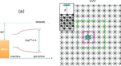
quasi-particle energy gap (Egap) of a molecule, defined as the difference between its ionization potential (I) and electron affinity (A), gets reduced with respect to that of the gas phase by adsorbing the molecule on a polarizable substrate. In a quasiparticle picture the I is negative of the highest occupied molecular orbital (HOMO) energy, while the A corresponds to the energy of the lowest unoccupied molecular orbital (LUMO). The reduction of theI andAof a molecule adsorbed on a metallic surface is mainly due to the Coulomb interaction between the added charge on the molecule and the screening electrons in the substrate. This interaction leads to a polarization of the surface, so that a surface charge with opposite sign with respect to the charge state of the molecule is formed. This nonlocal feature, called the image-charge effect, becomes more relevant as the molecule gets closer to the metallic surface. As a consequence, the reduction of theI and theA, hence of the HOMO-LUMO gap, becomes more prominent with the molecule approaching the surface, as schematically illustrated in Fig.1(a).
In general, conventional electronic structure theory strug-gles when predicting the level alignment at a metal/molecule interface, since only rarely are nonlocal correlation effects
explicitly included. This is, for instance, the case for density functional theory (DFT),6,7 today the most widely used
method for computing the electronic structure of materials. In particular, there are two important issues related to DFT and the problem of level alignment. On the one hand, since the Kohn-Sham eigenvalues cannot be rigorously interpreted as removal energies, Koopman’s theorem in general does not apply, so that the Kohn-Sham spectrum cannot be taken as a quasiparticle spectrum. The only exception is the HOMO (but not any of the HOMO-n levels), which can be associated with the negative of theI.8–10Even leaving interpretative issues aside,
in practice the Kohn-Sham energy levels often are not a good representation of the true excitation spectrum of a material, namely, they are not found at the correct energy position. On the other hand, in static DFT the standard approximations to the exchange and correlation functional, including the local density approximation (LDA),11hybrid functionals,12or explicitly self-interaction corrected ones,13,14 do not include,
or they do but just poorly, nonlocal correlation effects. This means that, although some of the functionals can predict with satisfactory accuracy the energy levels of the molecule in the gas phase, they all fail in describing properly the level renormalization as the molecule approaches the surface. For instance, in the LDA there is no change in the HOMO-LUMO gap as a molecule gets closer to a metallic surface.15
A conceptually straightforward way to include such nonlo-cal correlation effects in the description is that of using many-body perturbation theory, namely, the GW approximation constructed on top of DFT.16–18 This approach has been used
Alternatives to the GW approach, which to some degree also go beyond taking the simple DFT Kohn-Sham spectrum, include scissor operators (the DFT+ approach),24–29where
the HOMO and LUMO eigenvalues are shifted to match values obtained either from experimental data or from separate total energy difference calculations (SCF) plus classical image-charge models, and modifiedSCF schemes.30,31
Among the various possibilities constrained DFT (CDFT) represents a conceptually different approach to the problem. The idea behind CDFT is that one can always define an appropriate density functional, implementing a given desired constraint on the charge density32 (e.g., one can demand that an electron is localized on a particular group in a molecule). This is obtained by introducing an appropriate external potential in the Kohn-Sham equations. The crucial point is that the approach is fully variational, meaning that the energy minimum of the constrained functional represents the ground state of the system under that particular constraint.33–35 The method allows, for example, to access energies and electron density distributions of charge-transfer states of a given system, and has been successfully applied to the study of long-range charge-transfer excitations between molecules.33,36,37
In the present study we apply CDFT to the investigation of the energy-level alignment of metal/molecule interfaces. In relation to this problem, CDFT has two main advantages. First, since CDFT is based on total energy differences, it does not present the conceptual problems of interpreting the Kohn-Sham eigenvalues as a true quasiparticle spectrum. Second, one has to note that the total energy, even in the case of local functionals, is a rather accurate quantity, in contrast to the charge density that local functionals usually tend to overdelo-calize. This means that a theory that improves the charge den-sity but that relies on the total energy is expected to be accurate. The present paper is organized as follows. First we provide a description of the CDFT method used, with details on how the constrained is imposed. Then results for a specific system consisting of a benzene molecule deposited on a Li(100) surface are presented, focusing on charge-transfer energies, and hence level alignment. In particular, we evaluate the quantitative accuracy of the results as a function of the distance between the molecule and the surface, and its dependence on a set of parameters such as the system size and the boundary conditions (periodic versus finite). Towards the end we evaluate the changes in the electron density caused by the net charge on the molecule, and in particular we determine the position of the image-charge plane as a function of molecule-surface distance. We then use the calculated image-charge plane position in a classical model for the energy-level shifts and compare our ab initio energies to availableGWresults.
II. METHOD
In the Kohn-Sham (KS) framework7 the total energy (in atomic units) is given by
E[ρ]= α,β
σ Nσ
i
φiσ| −1 2∇
2|φiσ
+
dr vn(r)ρ(r)+J[ρ]+Exc[ρα,ρβ], (1)
whereJis the Hartree energy,Excis the exchange-correlation energy,vn(r) is the external potential,ρσ(r) is the electronic density for spinσ = ↑,↓ofNσelectrons (ρ=ρ↑+ρ↓), and the set{|φiσ}contains the KS wave functions that minimize the energy. A generic constraint on the charge density is that there is a specified number of electrons for each spinNcσwithin a certain region of space. This can be written as
wσc(r)ρσ(r)dr=Nσc, (2)
wherewσ
c(r) is a weighting function that describes the spatial extension of the constraining region. In the simplest case wσ
c(r) can be chosen to be equal to 1 within a certain volume and 0 elsewhere. In order to minimize the KS total energy of Eq.(1) subject to the constraint of Eq. (2), an additional spin-dependent term, proportional to the Lagrange multiplier Vσ
c, is added to the energy. A new functional is thus defined to be
W[ρ,Vc]=E[ρ]+ σ
Vcσ
wσc(r)ρσ(r)dr−Nσc
. (3)
When ρ satisfies the constraint in Eq. (2), then E[ρ]= W[ρ,Vc] by construction. Up to the ρ-independent term
σVcσNcσ,W[ρ,Vc] is the ground-state energy of a system with an additional spin-dependent external potentialVσ
c wσc(r). The KS equations with this extra potential are then given by
−1
2∇ 2+v
n(r)+vσxc(r)+V σ cw
σ c(r)+
ρ(r)
|r−r|dr
φσ i (r)
= iφσi(r), (4)
wherevσ
xcis the exchange and correlation potential. As in the standard Kohn-Sham DFT the electron density is constructed from the occupied Kohn-Sham eigenvectors {φiσ(r)} until consistency is achieved. In this particular case the self-consistency has to also guarantee that the constraint set by Eq. (2) is satisfied. The minimization then proceeds as follows. First, as in the standard Kohn-Sham scheme, an initial charge density is defined and then updated until the Kohn-Sham equations are satisfied self-consistently. Second, at every self-consistent step in this update of the charge density a second self-consistent loop is performed, where for a given input densityρ(r) the value ofVcσ is updated until the output charge density obtained via solution of Eq.(4) satisfies the constraint of Eq.(2). This second step is performed following an optimization scheme suggested in Ref.34. UpdatingVσ
c in this way ensures that at each self-consistent step and therefore also at convergence the constraint is fulfilled.
This methodology was implemented in the DFT package SIESTA.38SIESTAuses a linear combination of atomic orbitals (LCAO) basis set, so that, instead of defining the constraining region in real space via the functionwσ
c(r), we define it over the LCAO space. This means requiring that the total charge projected onto a given set of basis orbitals is equal toNcσ. For this aim we have implemented both the L¨owdin35,39 and the M¨ulliken40 projection schemes. A detailed description of the
Using such a CDFT approach we can evaluate the charge-transfer energy between the molecules and the metal surface, and hence the position of the frontier energy levels with respect to the Fermi energy of the metal. For a given substrate size and perpendicular distancedbetween the molecule and the surface atoms, first a standard DFT calculation without constraints is performed. This determines the total ground-state energy of the combined molecule+substrate system E(mol/sub;d) and the amount of charge present on each fragment, one fragment being the molecule and the other the substrate. In our calculations we considerdranging from 4 to 14 ˚A, where the molecule is only weakly coupled to the substrate, so that the amount of charge on each fragment is a well-defined quantity. Although CDFT is designed for arbitrary geometries and constraints, in the case of overlapping fragments the amount of charge localized on each fragment becomes ill defined and the results have to be taken with care.33
The next step consists in performing a different DFT calculation, where the constraint is set in such a way that one electron is removed from the molecule and one electron is added to the substrate. The total energy of such a charge-transfer state isE(mol+/sub−;d). Hence the charge-transfer energy needed to transfer one electron from the molecule to the substrateE+CTis given by
ECT+ (d)=E(mol+/sub−;d)−E(mol/sub;d). (5)
In an analogous way we obtain the charge-transfer energy gained by moving one electron from the surface to the molecule ECT− as
ECT−(d)=E(mol/sub;d)−E(mol−/sub+;d), (6)
whereE(mol−/sub+;d) is the CDFT ground-state energy of the configuration where one electron is moved from the metal surface to the molecule. We note that such a procedure always deals with globally charge neutral simulation cells, so that no monopole energy corrections are necessary under periodic boundary conditions. Moreover, for practical calculations the charge-transfer approach can be expected to be more accurate than a calculation using non-neutral cells, where the metal is kept neutral but the molecule is charged. For such non-neutral calculations the image charge is formed on the metal surface in an analogous way to the charge-transfer setup. However, in order for the metal cluster to be charge neutral, a charge with opposite sign will also form on the surface of the metallic cluster. Given the finite size of the cluster, this will lead to additional inaccuracies due to the interaction between the image charge and such a spuriously confined additional surface charge.
Within the charge-transfer procedure we can directly deter-mine the energy-level alignment at the interface, since−E+CT (−ECT− ) corresponds to the energy of the HOMO (LUMO) with respect to the substrate Fermi energy. In a similar constrained-DFT approach,31Sau and co-workers calculated the charging
energy associated with transferring small amounts of charge from the substrate to a specific molecular orbital. The charge-transfer energy was then obtained by extrapolation to integer charge. In order to avoid the use of such an extrapolation, here we always transfer an entire electron between the molecule and the substrate. Since a CDFT calculation has a computational cost only marginally more expensive than that of a standard
FIG. 1. (Color online) (a) Schematic energy-level diagram of the frontier orbitals of a molecule approaching a metallic surface. Note the HOMO-LUMO level renormalization as a function of the molecule-surface distancez due to polarization of the metal. (b) Top-view ball-stick representation of a benzene molecule at a Li(001) surface for a Li(001) 12×12 supercell. The dashed rectangles show the 3×3 (purple) and 6×6 (green) supercells. The inset in (b) is the side view of the benzene lying flat at a distancedfrom the surface. DFT ground-state one (the CPU time increases by about a factor of 2 over the entire self-consistent cycle), CDFT allows us the study of large organic molecules on surfaces. This is a prohibitive task for many-body-corrected quasiparticle schemes, such as theGWmethod.
We apply our CDFT method to compute the energy-level alignment of a benzene molecule as a function of its distance d from a Li(100) surface. The calculations are performed using norm-conserving relativistic pseudopotentials,41and the
LDA11for the exchange-correlation potential. The real-space
grid is set by an equivalent mesh cutoff of 300 Ry and the charge density, and all the operators are expanded over a double-ζ polarized basis set with an energy shift of 0.03 eV.38
The Li metallic surface is modeled by a 6 atomic layer thick slab. The bcc primitive unit cell lattice constant is set to 3.51 ˚A. We consider two types of boundary conditions in the plane of the Li substrate surface, namely, periodic boundary conditions (PBCs) and nonperiodic boundary conditions (non-PBCs). Furthermore, in order to investigate the finite size effects originating from the size of the Li surface, we consider three different cell sizes (for both PBCs and non-PBCs), namely, small (3×3 atoms per layer), intermediate (6×6), and large (12×12) (see Fig.1). In the case of non-PBCs the real-space box containing the Li slab supercell has dimensions 55×55×55 ˚A3. This is chosen in such a way that even for the 12×12 slab there is at least 15 ˚A of vacuum between the Li slab and the boundaries of the simulation box. By using a cubic box one can apply Madelung corrections in SIESTA. These are necessary since the electrostatic potential is calculated by using periodic boundary conditions.42 In the case of PBCs
the in-plane dimensions are set by the Li supercell size and thus are 10.56×10.56, 21.09×21.09, and 42.12×42.12 ˚A2, respectively, for the 3×3, 6×6, and 12×12 cell. The cell dimension in the direction perpendicular to the surface plane is the same as for the case of non-PBCs, namely, 55 ˚A.
[image:3.608.315.558.74.207.2]of this spurious interaction can be reduced by increasing the size of the unit cell. For the PBC setup the dimensions in the plane are set by the Li cluster size, while for non-PBC calculations we use a large simulation cell which minimizes the dipole-dipole interaction between periodic images. In this way we can disentangle the effects of changing the extension of the Li surface in plane from those associated with the size of the simulation box. Furthermore, in the case of non-PBCs, edge effects may arise and our aim is to find the required cluster and cell size that gives quantitatively accurate charge-transfer energies.
III. RESULTS
In order to determine the energy-level alignment between the molecule and the surface, we first need to determine the Li work function (WF). This is calculated by performing a simulation for the Li slab with PBCs and no benzene adsorbed and by taking the difference between the vacuum potential and the slab Fermi energy. The so obtained value for the Li(001)WFis 2.91 eV. This is in fair agreement with previous calculations (3.03 eV),43which have also shown that the LiWF can vary by about 0.5 eV depending on the crystallographic orientation of the surface. The experimental values reported for polycrystalline Li vary considerably (2.3–3.1 eV), as discussed in Ref.44and references therein.
[image:4.608.317.554.72.211.2]In this case of non-PBCs the Li substrate is essentially a giant molecule and we can calculate the I and the A by means of theSCF method, where I =E(N−1)−E(N) and A=E(N)−E(N+1) (N is the number of electrons in the neutral system). The results are listed in TableIfor the different Li cluster sizes. We note that there is a substantial difference between theIandA, resulting in a quasiparticle energy gap of the order of 1 eV for the Li clusters. Such a gap arises because of the charge confinement in the finite cluster. In this case electron-electron repulsion energy leads to a decrease of the Aand an increase of theI as compared to theWF calculated with PBCs. If instead of adding (removing) a full electron we add (remove) a small fractional charge (0.1 of an electron), electron-electron repulsion energy becomes negligible, the gap disappears, and we obtain A=3.0 eV (I =3.1 eV).
TABLE I. Ionization potential (I), electron affinity (A) and quasi particle gap (Egap), in eV, for the three Li substrates considered and for
the benzene molecule in the gas phase compared with experimental data and GW calculations.
Li substrates
3×3 6×6 12×12 Benzene gas phase
SCF SCF GW Expt.
I 3.46 3.44 3.55 9.56 9.23a/9.05b/7.9c 9.24d
A 1.57 2.18 2.63 −1.45 −0.80a/−1.51b/−2.7c −1.14e
Egap 1.89 1.26 0.92 11.01 10.51f/10.55b/10.6c 10.38
aReference48. bReference49. cReference20. dReference45. eReference46. fReference15.
5 10 15
d(Å)
-8-4 0 4
E
CT(eV)
3x3 6x6 12x12
5 10 15
d(Å)
-8 -4 0 4
E
CT(eV)
3x3 6x6 12x12
-(E-CT)
-(E+CT)
-(Imol-WF)
-(Amol-WF)
non-PBC PBC
(a) (b)
FIG. 2. (Color online) Negative of the charge-transfer energy ECT− and removal energyECT+ as a function of the molecule-surface distance d for the three clusters considered. (a) and (b) are for non-PBC and PBC calculations, respectively. The green dashed lines represent the negative of theImolandAmolof the isolated molecule
(SCF calculations) shifted by the calculated LiWFof 2.91 eV.
Likewise, the gap is reduced for larger cluster, in which the electron density of the additional electron (hole) can delocalize more. Before investigating the combined molecule/Li system we calculate also theI and the Afor the isolated benzene molecule, and our results are shown in TableI. We find the energy gap for the molecule in the gas phase,Egap=I −A, to be in good agreement with experiments,45,46 with other
works using the SCF (Ref. 47) approach, and with GW calculations.15,48
The benzene/Li interface [see Fig. 1(b)] consists of a benzene molecule, in its gas phase geometry, positioned parallel to the Li surface at a distanced. We now evaluate the dependence of the various charge-transfer energies (positions of the HOMO and LUMO) on d for all the different Li supercells as well as for both non-PBCs and PBCs. We start by presenting our results for calculations performed with non-PBCs. In Fig.2(a)we plot −E+CT and−ECT− as a function ofdfor all three Li clusters considered. As expected, due to the electron-hole attraction, the absolute value of the charge-transfer energy decreases asd gets smaller. This in itself shows that CDFT can capture nonlocal Coulomb contributions to the energy. While for small d the energies of the three different clusters are approximately equal to each other, for large distances they differ significantly. In order to determine the origin of such deviations we evaluate the same energies in the limit of very large distances (d → ∞), where
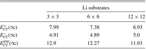
TABLE II. Charge-transfer energies (in eV) in the limit of large distances (d→ ∞) for the three molecule/Li cluster cells investigated. Values are obtained by evaluating Eqs.(7)–(9)with theI sandAstaken from TableI.
Li substrates
3×3 6×6 12×12
ECT+(∞) 7.99 7.38 6.93
ECT−(∞) 4.91 4.89 5.0
[image:4.608.314.560.669.752.2]they become
ECT+(∞)=Imol−ALi (7)
and
ECT− (∞)=Amol−ILi, (8)
since the interaction energy between the charge on the Li slab and that on the molecule vanishes ford → ∞. The charge-transfer energy gap is then given by
ECTgap(∞)=E+CT(∞)−ECT−(∞)
=Imol−Amol+(ILi−ALi). (9) WhileImolandAmolare independent of the cluster size, this is not the case forILiandALi(see TableI). This reflects in the fact that the charge-transfer energies at a large molecule-surface separation cary with the cluster size (see TableII).
At large distances the variation of ECT+ with the Li cluster sizes is mainly caused by significant changes in ALi. Interestingly, this is not the case for E−CT, sinceILi is approximately the same for all the Li clusters considered. As d gets smaller, the extension of the image charge on the Li slab is reduced, so that even small clusters are large enough to contain most of the image charge. Therefore the energy differences depend less on the cluster size. Ford up to about 6 ˚A, Fig.2(a)shows thatECT+ andECT− are converged even for the small 3×3 supercell. Since in organic-based devices the first molecular layer deposited on top of the metallic substrate is typically rather close to the surface, we expect that in these situations a rather small cluster size will be already sufficient for our CDFT scheme to yield an accurately converged level alignment. This means that the CDFT approach is a valuable tool for an accurate evaluation of the electronic structure of molecules on surfaces in realistic conditions. Finally, when one looks at largerd, it is immediately clear that larger cluster sizes must be considered. The green dashed lines in Fig. 2
correspond to the infinite cluster size limit, for which we have ILi=ALi=WF ≈2.9 eV. It can then be seen that, even up to the largest consideredd of 14 ˚A, results obtained for the 12×12 cluster are within the infinite cluster limit (set in the figure by the two green dashed lines), so that they can be considered converged.
We now move to the case of PBCs, in which there are no edge effects due to the finite size of the cell. Results for the charge-transfer energies are presented in Fig.2(b). Although the general trends are analogous to the ones found for the case of non-PBCs, we note that for the 3×3 supercell the changes in the charge-transfer energy as a function of d are largely overestimated. This is due to the use of PBCs, in which the lateral dimensions of the supercell box coincide with those of the Li slab (i.e., there is no vacuum). Because of the PBCs one effectively simulates a layer of charged molecules and not a single molecule on the surface. Thus, when the molecules are closely spaced, the charge-transfer energy is that of two opposite charged surfaces facing each other (the molecular layer and the Li slab). This is significantly larger than that of a single molecule (note that we always compare the charge-transfer energy per cell, i.e., per molecule). When one increases the size of the supercell and arrives at 12×12, both PBC and non-PBC calculations produce the same results. This confirms
the observation that the 12×12 supercell is large enough to contain a substantial part of the image charge as well as to minimize the Coulomb interaction between repeated supercell images up tod=14 ˚A.
From the charge-transfer energies we can now obtain an approximate value of the energies of the HOMO and LUMO orbitals, by offsetting them with the metal WF, so that EHOMO −(ECT+ +WF) and ELUMO −(ECT− +WF). Note that if the metal substrate is semi-infinite in size, then these relations become exact, since by definition the energy required to remove an electron from the metal and that gained by adding it are equal to the work function. However, in a practical calculation, a finite size slab is used, and therefore the relations are only approximately valid due to the inaccuracies in the calculatedWF for finite systems. As shown above, the WF becomes more accurate as the cluster size is increased.
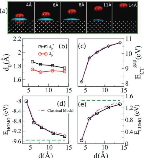
In Figs.3(d)and3(e)we show the calculated values for the 12×12 supercell and PBCs obtained by using the LiWFof the infinite slab of 2.91 eV, and in Fig.3(c)we presentECTgap(d)= ECT+(d)−ECT−(d). In order to quantify how the image charge changes the charge-transfer energies as a function ofd, we
FIG. 3. (Color online) Image-charge analysis. (a) Isosurface of the difference between the charge densities calculated with DFT (ground state) and CDFT (charge-transfer state) ρ(r). Note the formation and the spatial distribution of the image charge. Different panels correspond to different molecule/surface distances d. The isosurfaces are taken at 10−4e/A˚3. Red isosurfaces denote negative
ρ(r) (electron depletion), while blue are for positiveρ(r) (electron excess). (b) Position of the charge image plane taken from the surface atoms [see Eq.(11)], respectively, when one electron, d0+, or one
hole,d0−, is transferred from the molecule to the Li substrate for the 12×12 PBC calculations as a function ofd. (c)–(e) areEgapCT,EHOMO,
andELUMO, respectively, as a function ofdand compared with the
classical model of Eq.(10). The dashed green lines are−Imol and
[image:5.608.316.560.322.590.2]can writeE±CT(d)=ECT±(∞)+V(d), where the new quantity V(d) corresponds to the energy lowering due to the distance-dependent electron-hole attraction. It was demonstrated a long time ago,50 by using self-consistent DFT calculations, that for flat surfacesV(d) can be accurately approximated by the classical image-charge energy gain
V(d)= −q 2
4(d−d0)
, (10)
where q is the charge on the molecule, andd0 is the height of the image-charge plane with respect to the topmost surface atomic layer
d0(d)= dB
dA z ρxy(z;d)dz
dB
dA ρxy(z;d)dz
. (11)
In other words,d0can be interpreted as the center of gravity of the screening charge density localized on the metal surface, and in general it depends ond. Hereρxy(z;d)= dxdyρ(r;d) andρ(r;d) is the difference between the charge densities of the DFT (ground state) and the CDFT (charge-transfer state) solutions for a fixed d. Note that the charge transfer between the surface and the molecule leads to the formation of a spurious charge layer on the back side of the Li slab (i.e., opposite to the surface where the molecule is placed), which is due to the finite number of atomic layers used to simulate the metal surface. In order not to consider such a spurious charge while evaluating the integral in Eq.(11), the two integration limits, dA anddB, are chosen in the following way: (1)dA is taken after the first twoρ(d) charge oscillations on the back of the cluster, and (2)dB is the distance at whichρ(d) changes sign between the top Li layer and the molecule (i.e., it is in the vacuum).
Figure3(a)provides a visual representation of the image-charge formation as the molecule approaches the surface and shows isosurface plots of ρ(r;d) for different distancesd. Here we present the case in which one electron is removed from the molecule and is added to the Li surface. As one would expect, the farther away the molecule is from the surface, the more delocalized the image charge becomes.50
Note that the isosurface value is kept constant for all d [ρ(r;d)=10−4e/A˚3], so that the apparent shrinking of the image charge ford =11 ˚A simply reflects the fact that most of the image charge is now spread at an average density smaller than 10−4 e/A˚3. Likewise, no isosurface contour appears on the Li slab ford =14 ˚A, since now the image charge is rather uniformly spread at low density. In contrast, at small d the oscillations of the charge density between the atomic layers of the metallic surface can also be seen. It can also be seen that at 4 ˚A the charges on the molecule and the image charge on the Li surface start to overlap. Note that for even shorter distances, when the overlap becomes very large, the CDFT approach presented here becomes ill defined, since the charge on each fragment is not well defined anymore.
By evaluating Eq.(11) we now determined0(d) and the results obtained for the 12×12 PBC calculations are shown in Fig.3(b)for both electron (d0+) and hole (d0−) transfer from the molecule to the surface. The averaged0values are 1.81 and 1.72 ˚A ford0+andd0−, respectively. Although the two values are similar, they are not identical. This is consistent with the
small band gap of the Li slab, which indicates that holes and electrons behave differently. The average values ofd0+andd0− can now be used to evaluate Eq.(10)for the classical model. The results are shown in Figs.3(c)–3(e)and demonstrate that the classical model works remarkably well for this system [the calculated slope of both EHOMO(d) andEHOMO(d) matches almost perfectly that obtained by CDFT]. It also shows once again that the results for our 12×12 PBC cell are indeed well converged with respect to the slab and cell size.
Finally we make a comparison between our results and those available in the literature for many-body-based calcula-tions. We find an overall reduction ofECTgap of 2.5 eV, when the benzene moves from infinity tod=4.5 ˚A. Garcia-Lastra et al.20 studied the dependence of the frontier quasiparticle
energy levels of a benzene molecule as a function of the distance to a Li substrate by means ofGWcalculations. They found an overall reduction inEgapof∼3.2 eV as compared to the benzene HOMO-LUMO gap in the gas phase, as one can extract from Fig. 1(c) of Ref.20. The authors also fit theirGW results to the classical model, finding the best match fitting for d0=1.72 ˚A, in very good agreement with our calculated value. There is a small discrepancy in the results of Ref.20, since if one uses the classical model of Eq.(10)withd0=1.72 ˚A, then the HOMO-LUMO gap reduction should be smaller than 3.2 eV, namely, 2.6 eV atd =4.5 ˚A. Note that theGWresults are obtained for cells much smaller than the converged 12×12 used here. If we now force the classical model to fit our results for the 3×3 and 6×6 supercells, we will obtain, respectively, d0=2.3 and 2.1 ˚A for a corresponding gap reduction of 3.27 and 3.0 eV. In these two cases, however, the fit is good at all d only for the 6×6 supercell, while it breaks down for the 3×3 one fordbeyond 8 ˚A. This is somehow expected since for large molecular coverages (the 3×3 cell) the pointlike classical approximation is no longer valid.
IV. CONCLUSION
gives a direct way of determining the position of the image charge for such interfaces. Overall, CDFT applied to the level alignment problem appears as a promising tool for characterizing theoretically organic/inorganic interfaces, so that it has a broad appeal in fields such as organic electronics, solar energy devices, and spintronics.
ACKNOWLEDGMENTS
The authors are thankful to the King Abdullah University of Science and Technology (Kingdom of Saudi Arabia) for financial support through the ACRAB project and to the Trinity College High-Performance Computer Center for computational resources.
APPENDIX: IMPLEMENTATION DETAILS
Our implementation of the constrained-DFT approach withinSIESTAfollows the prescription of Wuet al.described in Ref.51. Accordingly, we begin by defining a set of constraints on the electronic spin density of the form
σ
wσk(r)ρσ(r)dr−Nk=0, (A1)
wherein σ = ↑,↓ represents the spin index, wσ
k(r) is a weight function corresponding to the constraint k, defining the property being constrained, andNkis the constraint value. The total electron density is given by
ρ(r)= σ
ρσ(r)= σ
Nσ
i
φσi(r)2, (A2)
where Nσ is the number of occupied Kohn-Sham orbitals φσi(r). A Lagrange multiplier Vk is associated with each constraint specified in Eq. (A1). This allows the following modified energy functional to be defined,
W[ρ,{Vk}]=E[ρ]+ k Vk σ
wσk(r)ρσ(r)dr−Nk
,
(A3)
with E[ρ] being the standard Kohn-Sham (KS) energy functional given by
E[ρ]= σ
Nσ
i
φiσ−1 2∇
2φσ i
+
vext(r)ρ(r)
+J[ρ]+Exc[ρ↑,ρ↓]. (A4) In Eq.(A4)the first term is the kinetic energy,vext(r) is the external potential,J[ρ] is the classical Coulomb energy, and Exc[ρ↑,ρ↓] is the exchange-correlation energy. The variational principle yields the stationary condition for the functionalW with respect to the normalized orbitalsφσ
i, which leads to the following modified Kohn-Sham equations,
−1
2∇
2+vext(r)+
dr ρ(r
) |r−r|+v
σ xc(r)
+
k
Vkwσk(r)
φiσ(r)= σiφ σ
i(r). (A5)
Thus the constraints enter the effective KS Hamiltonian in the form of an additional external potentialkVkwσk(r). The ground state of the constrained KS system is obtained by solving Eq.(A5)in conjunction with Eq.(A1). Wuet al.have shown51 that the functionalW is concave with respect to the
parametersVk, and that by optimizingWthrough varying{Vk}, one can find the constraint potential that yields the ground state of the constrained system. In order to optimizeW, we utilize its first derivate with respect to{Vk}given by
dW dVk = σ Nσ i δW δφiσ
∂φiσ ∂Vk +c.c. +∂W ∂Vk = σ
wkσ(r)ρσ(r)dr−Nk, (A6)
where the stationary conditionδφδWσ
i =0 implied by Eq.(A5)is
used. Thus we see that the derivative dWdV
k vanishes
automati-cally when Eq.(A1)is satisfied.
We now outline the implementation of this formalism for the simulation of electron transfer processes withinSIESTA. In a typical electron transfer problem one has to partition the system into a donor region (D) and an acceptor region (A). WithinSIESTA, this is done by specifying a certain group of atoms as belonging to D and a second group of atoms as belonging to A. The constrained calculation then involves the transfer of a specified amount of charge from D to A. In order to partition the continuous electron density in real space between the A and D regions, we choose an appropriate population analysis scheme, which in turn determines the form of the weight functionwkin Eq.(A1). The localized numerical orbital basis set within SIESTA is particularly suitable for atomic-orbital-based population analysis schemes such as the ones due to Lowdin39and Mulliken.40We have implemented weight functions corresponding to both the Lowdin and Mulliken schemes withinSIESTA. For L¨owdin populations, the number of electrons on a group of atomsCis given by
NC =
μ∈C
S12DS 1 2 μμ= νλ Dνλ
μ∈C S 1 2 λμS 1 2
μν=Tr
DwLC
,
(A7)
whereDandSare the density and overlap matrices, respec-tively, andwL
Cλν=
μ∈CS
1 2
λμS
1 2
μν defines the L¨owdin weight matrix. Similarly, with a Mulliken population analysis, the number of electrons on a group of atomsCis
NC=
μ∈C
[D(S)]μμ =Tr[(DS)], (A8)
with the corresponding weight matrix given by
wCμνM = ⎧ ⎪ ⎨ ⎪ ⎩
Sμν ifμ∈C andν∈C, 1
2Sμν ifμ∈C orν ∈C, 0 ifμC andνC.
For charge-transfer problems, Wuet al.recommend a parti-tioning of the charge density based on the L¨owdin scheme.
is similar to a conventional SCF cycle wherein the orbitals obtained by solving the KS equations and the associated self-consistent density are updated. The inner loop consists of optimizing theVkmultipliers to ensure that the constraint condition given in Eq. (A1) is satisfied at each step of the outer loop. By Eq. (A6), this is equivalent to finding the extremes of W. Since the derivative of W with respect to the Vk is readily available from Eq. (A6), we employ a conjugate gradient (CG) optimization procedure to ensure that Eq. (A1) is satisfied. Subsequently, the KS equations are solved and the resulting orbitals are used to update the KS density and Hamiltonian in the outer loop. We note that Wuet al.also calculated the second derivative (Hessian matrix) ofWwith respect to theVkparameters and employed Newton’s method to optimize{Vk}. However, the expression for the second derivatives∂V∂W
k∂Vl depends explicitly on the KS
orbitals, whereas the first derivative [Eq.(A6)] involves only the density.51 We therefore prefer to work with the gradient alone and employ a CG optimization scheme for the {Vk}. Thus the overall SCF procedure consists of the following sequence of steps: (i) Construct the standard KS Hamiltonian
Hfor the current guess density. (ii) Obtain the constrained KS HamiltonianHC =H+
kVkwσk(r) by adding the constraint potentialkVkwkσ(r) from the previous iteration. (iii) Using the Pulay scheme, mixHcwith Hamiltonians from previous iterations to obtain HC. (iv) By keeping HC fixed, opti-mize {Vk}so that the constraints in Eq. (A1) are satisfied. (v) Solve the KS equations for the Hamiltonian combining
HC and the optimized {Vk}. The new density matrix D thus obtained and the optimized {Vk} are used in the next iteration. (vi) Repeat steps (i)–(v) until self-consistency is achieved.
*Present address: Lawrence Berkeley National Laboratory, University
of California, Berkeley, California 94720, USA.
1N. Koch,Chem. Phys. Chem.8, 1438 (2007).
2R. Hesper, L. H. Tjeng, and G. A. Sawatzky,Europhys. Lett.40, 177 (1997).
3J. Repp, G. Meyer, S. M. Stojkovi´c, A. Gourdon, and C. Joachim, Phys. Rev. Lett.94, 026803 (2005).
4X. Lu, M. Grobis, K. H. Khoo, S. G. Louie, and M. F. Crommie, Phys. Rev. B70, 115418 (2004).
5M. T. Greiner, M. G. Helander, W.-M. Tang, Z.-B. Wang, J. Qiu,
and Z.-H. Lu,Nat. Mater.11, 76 (2011).
6P. Hohemberg and W. Kohn,Phys. Rev.136, B864 (1964). 7W. Kohn and L. J. Sham,Phys. Rev.140, A1133 (1965). 8J. F. Janak,Phys. Rev. B18, 7165 (1978).
9J. P. Perdew, R. G. Parr, M. Levy, and J. L. Balduz,Phys. Rev. Lett. 49, 1691 (1982).
10J. P. Perdew and M. Levy,Phys. Rev. Lett.51, 1884 (1983). 11D. M. Ceperley and B. J. Alder,Phys. Rev. Lett.45, 566 (1980). 12A. D. Becke,J. Chem. Phys.98, 1372 (1993).
13C. D. Pemmaraju, T. Archer, D. S´anchez-Portal, and S. Sanvito, Phys. Rev. B75, 045101 (2007).
14A. Filippetti, C. D. Pemmaraju, S. Sanvito, P. Delugas, D. Puggioni,
and V. Fiorentini,Phys. Rev. B84, 195127 (2011).
15J. B. Neaton, M. S. Hybertsen, and S. G. Louie,Phys. Rev. Lett.97, 216405 (2006).
16J. C. Inkson,J. Phys. C: Solid State Phys.6, 1350 (1973). 17M. S. Hybertsen and S. G. Louie, Phys. Rev. B 34, 5390
(1986).
18G. Onida, L. Reining, and A. Rubio, Rev. Mod. Phys.74, 601 (2002).
19J. M. Garcia-Lastra and K. S. Thygesen, Phys. Rev. Lett. 106, 187402 (2011).
20J. M. Garcia-Lastra, C. Rostgaard, A. Rubio, and K. S. Thygesen, Phys. Rev. B80, 245427 (2009).
21I. Tamblyn, P. Darancet, S. Y. Quek, S. A. Bonev, and J. B. Neaton, Phys. Rev. B84, 201402 (2011).
22G.-M. Rignanese, X. Blase, and S. G. Louie,Phys. Rev. Lett.86, 2110 (2001).
23M. Strange and K. S. Thygesen,Phys. Rev. B86, 195121 (2012).
24A. Ferretti, A. Calzolari, R. Di Felice, and F. Manghi,Phys. Rev. B 72, 125114 (2005).
25S. Y. Quek, H. J. Choi, S. G. Louie, and J. B. Neaton,ACS Nano5, 551 (2011).
26V. M. Garc´ıa-Su´arez and C. J. Lambert,New J. Phys.13, 053026 (2011).
27S. Y. Quek, L. Venkataraman, H. J. Choi, S. G. Louie, M. S.
Hybertsen, and J. B. Neaton,Nano Lett.7, 3477 (2007).
28D. J. Mowbray, G. Jones, and K. S. Thygesen,J. Chem. Phys.128, 111103 (2008).
29E. Abad, J. Ortega, Y. J. Dappe, and F. Flores,Appl. Phys. A95, 119 (2008).
30J. Gavnholt, T. Olsen, M. Engelund, and J. Schiøtz,Phys. Rev. B 78, 075441 (2008).
31J. D. Sau, J. B. Neaton, H. J. Choi, S. G. Louie, and M. L. Cohen, Phys. Rev. Lett.101, 026804 (2008).
32P. H. Dederichs, S. Blugel, R. Zeller, and H. Akai,Phys. Rev. Lett. 53, 2512 (1984).
33B. Kaduk, T. Kowalczyk, and T. Van Voorhis,Chem. Rev.112, 321 (2012).
34Q. Wu and T. Van Voorhis,Phys. Rev. A72, 024502 (2005). 35Q. Wu and T. Van Voorhis,J. Phys. Chem. A110, 9212 (2006). 36Q. Wu and T. Van Voorhis,J. Chem. Phys.125, 164105 (2006). 37S. Yeganeh and T. Van Voorhis, J. Phys. Chem. C 114, 20756
(2010).
38M. Soler, E. Artacho, J. D. Gale, A. Garc´ıa, J. Junquera,
P. Ordej´on, and D. Sanchez Portal,J. Phys.: Condens. Matter14, 2745 (2002).
39P.-O. L¨owdin,J. Chem. Phys.18, 365 (1950). 40R. S. M¨ulliken,J. Chem. Phys.23, 1833 (1955).
41N. Troullier and J. L. Martins,Phys. Rev. B43, 1993 (1991). 42G. Makov and M. C. Payne,Phys. Rev. B51, 4014 (1995). 43K. Kokko, P. T. Salo, R. Laihia, and K. Mansikka,Phys. Rev. B52,
1536 (1995).
44N. D. Lang and W. Kohn,Phys. Rev. B3, 1215 (1971).
45L. A. Chewter, M. Sander, K. Muller-Dethlefs, and E. W. Schlag, J. Chem. Phys.86, 4736 (1987).
46J. C. Rienstra-Kiracofe, G. S. Tschumper, H. F. Schaefer, S. Nandi,
47J. C. Rienstra-Kiracofe, C. J. Barden, S. T. Brown, and H. F.
Schaefer,J. Phys. Chem. A105, 524 (2001).
48H.-V. Nguyen, T. A. Pham, D. Rocca, and G. Galli,Phys. Rev. B 85, 081101 (2012).
49G. Samsonidze, M. Jain, J. Deslippe, M. L. Cohen, and S. G. Louie, Phys. Rev. Lett.107, 186404 (2011).
50N. D. Lang and W. Kohn,Phys. Rev. B7, 3541 (1973).