Improving Density based Clustering using Metric Optimization

Improving Density-based Clustering using Metric

Optimization

Wesam M. Ashour

Islamic University of Gaza Gaza - Palestine

Islam A. Mezied

Islamic University of Gaza Gaza - Palestine

Abdallatif S. Abu-Issa

Birzeit University, West Bank – Palestine

ABSTRACT

Density-based clustering is one of the most important sciences nowadays. A various number of datasets depend on it. Since homogeneous clustering may generate a large number of smaller useless clusters, a good clustering method should give the permission to a significant density variation. This paper focuses on enhancing the clustering results after using density-based cluster algorithms DBSCAN (Density-density-based spatial clustering of applications with noise) or OPTICS (Ordering points to identify the clustering structure) by using statistical models. The use of statistical models supports improving results by reducing the number of noise points with the same cluster number and expand the selected area as recognized as cluster.

Keywords

Density-based, DBSCAN, OPTICS, Statistical, Selection model

1.

INTRODUCTION

Cluster analysis stands as one of the most significant and influential sciences these days. It tries to bring a group of properties together and then classify them into one group. This is valuable in the fields of data mining, statistics, and data analysis. The techniques of clustering are applied in many fields such as image processing, pattern recognition, machine learning, and information retrieval and others more. [1][2]

As mentioned earlier, clustering is analyzing the data into groups of related objects. There are various approaches to data clustering that differ in their complexity and influence, due to the huge number of applications that the algorithms have. For instance, from a machine learning perspective, clusters correspond to hidden patterns, the search for clusters is an independent learning, and the resulting system represents a data concept. On the other hand, from a practical perspective, clustering performs an important role in data mining applications such as scientific data exploration, information retrieval and text mining, spatial database applications, web analysis, marketing, medical diagnostics, computational biology, and many others. Although there has been a large amount of research into the role of clustering, nowadays-popular clustering methods often lose the chance to find high-quality clusters.

It is worthy to mention that Driver established cluster analysis in anthropology and Kroeber in 1932, brought in to psychology by Zubin in 1938 and Robert Tryon in 1939, and used by Cattell in 1943 in personality psychology.

There are two main types of clustering algorithms: partitioning and hierarchical algorithms. To begin with, partitioning algorithms build a partition of a database of objects into a set of clusters.

is an input parameter for these algorithms. The partitioning algorithm usually begins with an initial partition of and then uses an iterative control strategy to optimize an objective

function. Each cluster is represented by the gravity center of the cluster (k-means algorithms) or by one of the cluster objects located near its center (k-medoid algorithms( .

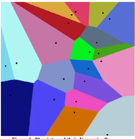
Partitioning algorithms use a two-step procedure. First, determine representatives minimizing the objective function. Second, appoint each object to the cluster with its representative “closest” to the considered object. The second step indicates that a partition is equivalent to a voronoi diagram and each cluster is embodied in one of the voronoi cells as shown in Figure 1 [3].

Correspondingly, the shape of all clusters found by a partitioning algorithm is convex, meaning it is very restrictive. Secondly, hierarchical algorithms build a hierarchical decomposition of . The hierarchical decomposition is presented by a dendrogram as shown in Figure 2, a tree that splits in repetition into smaller subsets until each subset contains only one object. In this type of a hierarchy, each node of the tree represents a cluster of .

Figure 1: 20 points and their Voronoi cells

Figure 2: Hierarchical clustering and dendrogram. 5 data points are clustered, and the dendrogram on the right side shows the clustering result. The height of each subtree

represents the distance between the two children

Figure 3: Samples of Density-based clustering

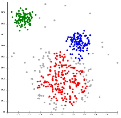
Density-based cluster is used in clustering analysis; it depends on locating big groups into smaller sets of groups depending on the density of the group as shown in Figure 3. A Density-based approach is to identify clusters in k-dimensional point sets. The data set is partitioned into a number of non-overlapping cells and histograms are constructed. Cells that have relatively high frequency counts of points are called the potential cluster centers and the boundaries between clusters are located in the “valleys” of the histogram. This method is capable of identifying clusters of any shape.

However, the space and run-time requirements for storing and searching multidimensional histograms can be excessive. Even if the space and run-time requirements are optimized, the performance of such an approach mainly depends on the size of the cells [3]. Therefore, it can find out the clusters of different shapes and sizes from a large amount of data, which is containing noise and outliers. On the other hand, it fails to manage the local density variation that exists within the cluster [4]. The most common and used algorithm is DBSCAN (Density-based spatial clustering of applications with noise). It was proposed by Martin Ester, Hans-Peter Kriegel, Jörg Sander and Xiaowei Xu in 1996.

Using Density-based clustering has various benefits as:

 Clusters can have arbitrary shape and size.

 Number of clusters is determined automatically.  Can separate clusters from surrounding noise.  Can be supported by spatial index structures.

Clustering of any type of data depends on the definition of a similarity or of a distance measure. The Euclidean distance is one of the popular distance measures, and a famous choice in time series clustering. The Euclidean distance measure is a special case of a norm. Norms may fail to hold similarity well when being applied [5].

It worth mentioning that clusters cannot only be defined based on the density attractors or modes but also as regions that are continuously above a threshold [6]. Such a definition give the permission to multiple attractor regions to be connected into one arbitrarily shaped cluster.

In the next section, more about density-based algorithms will be discussed and how they work and implemented, section three will introduce statistical models and focuses on more details about the selection model. Then in section four, we will explain our proposed work that describes how the statistical models were employed to improve the quality of applying density-based algorithms for clustering data. Section 5 discuss the experimental procedural and technical properties used for enhancing the outcome and compare the results. Finally, the conclusion will summarize the result and which quality metric of statistical models get the best case of solution.

2.

RELATED WORK

The DBSCAN (Density-based Spatial Clustering of Applications with Noise) is a trend algorithm of Density-based clustering. It involves two input parameters, (the radius of the cluster) and MinPts (the minimum data objects required inside the cluster). The DBSCAN burdens the responsibility of choosing parameter values that will bring on the discovery of acceptable clusters. An object is said to be core if it has (closed) -neighborhood. These parameter settings are usually experimentally set and difficult to determine. DBSCAN does not determine upper limit of a core object. As a result, the clusters detected by it, are having a broad variation in local density and forms clusters of any arbitrary shape [4].

Definition:Density Reachability - A point "p" is said to be density reachable from a point "q" if point "p" is within ε distance from point "q" and "q" has sufficient number of points in its neighbors, which are within distance ε.

Definition: Density Connectivity - A point "p" and "q" are said to be density connected if there exist a point "r" which has sufficient number of points in its neighbors and both the points "p" and "q" are within the ε distance. This is chaining process. So, if "q" is neighbor of "r", "r" is neighbor of "s", "s" is neighbor of "t" which in turn is neighbor of "p" implies that "q" is neighbor of "p".

The clusters are defined in such a way that they are unions of -neighborhoods of core points and two core points belong to the same cluster if and only if one of them is density reachable from the other one; recall that an object y is density reachable from x provided there are core points.

Such that for every and . Objects such that does not contain any core point are called noise objects; these objects do not belong to any cluster.

means that essentially different clusters can be joined together. To defeat these difficulties, in [7] the authors proposed OPTICS (Ordering Points to Identify the Clustering Structure) algorithm. Analogously as DBSCAN, also OPTICS depends on the distance and two parameters max and . However, unlike DBSCAN, OPTICS is not a clustering algorithm. Its purpose is to order all objects in such a way that closest objects (according to the distance ) become neighbors in the ordering.

This is accomplished by defining the so-called core-distance

and reachability-distance for every object .

OPTICS guarantees that, for every , if then belongs to the same -DBSCAN cluster as its predecessor. Thus, for any given , the -DBSCAN clusters correspond to the maximal intervals in the OPTICS ordering such that for every , but the first object of the interval. Regarding the choice of max, if it is too small, OPTICS cannot extract information about clustering structure. On the other hand, with growing max the runtime complexity of OPTICS grows greatly. Growing effort was committed to the choice of the density threshold for DBSCAN and OPTICS [8].

3.

STATISTICAL MODEL

A probability model is a useful concept for making sense of observations by regarding them as realizations of random variables, but the model that we can think of as having given rise to the observations is usually too complex to be described in every detail from the information available.

A statistical model embodies a set of assumptions concerning the generation of the observed data, and similar data from a larger population. A model represents, often in considerably idealized form, the data-generating process. The model assumptions describe a set of probability distributions, some of which are assumed to adequately approximate the distribution from which a particular data set is sampled.

A model is usually specified by mathematical equations that relate one or more random variables and possibly other non-random variables.

The necessity of introducing the concept of model selection has been recognized as one of the important technical areas, and the problem is posed on the choice of the best approximating model among a class of competing models by a suitable model selection criterion given a dataset. Model selection is the task of selecting a statistical model from a set of candidate models, given data. In the simplest cases, a pre-existing set of data is considered. However, the task can also involve the design of experiments such that the data collected is well-suited to the problem of model selection. Given candidate models of similar predictive or explanatory power, the simplest model is most likely to be the best choice. Model selection criteria are figures of merit, or performance measures, for competing models. In this paper, we shall briefly study the basic underlying idea of Akaike's information criterion (AIC), Bayesian Information Criterion (BIC), Residual Sum of Squares (RSS), and F-Measure score (F1).

a.

Akaike's information criterion

The Akaike information criterion (AIC) is a measure of the relative quality of a statistical model for a given set of data. That is, given a collection of models for the data, AIC estimates the quality of each model, relative to each of the other models. Hence, AIC provides a means for model selection.

AIC is founded on information theory: it offers a relative estimate of the information lost when a given model is usedto represent the process that generates the data. In doing so, it deals

with the trade-off between the goodness of fit of the model and the complexity of the model.

AIC does not provide a test of a model in the sense of testing a null hypothesis; i.e. AIC can tell nothing about the quality of the model in an absolute sense. If all the candidate models fit poorly, AIC will not give any warning of that.

Suppose that we have a statistical model of some data. Let L be the maximized value of the likelihood function for the model; let k be the number of estimated parameters in the model. Then the AIC value of the model is the following

Given a set of candidate models for the data, the preferred model is the one with the minimum AIC value. Hence AIC rewards goodness of fit (as assessed by the likelihood function), but it also includes a penalty that is an increasing function of the number of estimated parameters. The penalty discourages over fitting (increasing the number of parameters in the model almost always improves the goodness of the fit).

b.

Bayesian Information Criterion

BIC is a criterion for model selection among a finite set of models; the model with the lowest BIC is preferred. It is based, in part, on the likelihood function and it is closely related to the Akaike information criterion (AIC).

When fitting models, it is possible to increase the likelihood by adding parameters, but doing so may result in over fitting. Both BIC and AIC resolve this problem by introducing a penalty term for the number of parameters in the model; the penalty term is larger in BIC than in AIC.

The BIC is formally defined as

The BIC generally penalizes free parameters more strongly the Akaike information criterion, though it depends on the size of n and relative magnitude of n and k.

It is important to keep in mind that the BIC can be used to compare estimated models only when the numerical values of the dependent variable are identical for all estimates being compared. The models being compared need not be nested, unlike the case when models are being compared using an F-test

c.

Residual Sum of Squares

In statistics, the residual sum of squares (RSS) is the sum of squares of residuals. It is also known as the sum of squared residuals (SSR) or the sum of squared errors of prediction (SSE). It is a measure of the discrepancy between the data and an estimation model. A small RSS indicates a tight fit of the model to the data. In general,

Total sum of squares = explained sum of squares + residual sum of squares. In a model with a single explanatory variable, RSS is given by:

Where is the value of the variable to be predicted, is the _{value of the explanatory variable, and is the predicted}

d.

F-Measure score

In statistical analysis of binary classification, the F1 score (also F-score or F-measure) is a measure of a test's accuracy. It considers both the precision p and the recall r of the test to compute the score: p is the number of correct positive results divided by the number of all positive results, and r is the number of correct positive results divided by the number of positive results that should have been returned. The F1 score can be interpreted as a weighted average of the precision and recall, where an F1 score reaches its best value at 1 and worst score at 0.

The F-measure of the system is defined as the weighted harmonic mean of its precision and recall, that is,

Where the weight α [0, 1]. The balanced F-measure, commonly denoted as F1 or just F, equally weighs precision and recall, which means α = . The F1 measure can be written as

The F-measure can be viewed as a compromise between recall and precision. It is high only when both recall and precision are high. It is equivalent to recall when α = 0 and precision when α = 1. The F-measure assumes values in the interval [0, 1]. It is 0 when no relevant documents have been retrieved, and is 1 if all retrieved documents are relevant and all relevant documents have been retrieved.

4.

PROPOSED WORK

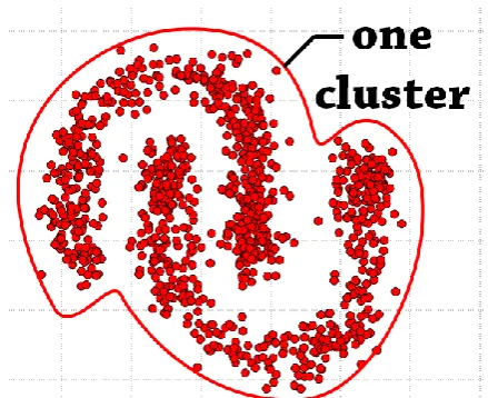
In this section of the paper we shed light on the process of enhancing the outcome of the clustering data after applying the density-based algorithms. This process is called post-processing, which means that the proposed work is not executed on density-based algorithms themselves, but the execution happens after getting the first result. The purpose behind using the proposed work is to cover some the leak coming from applying DBSCAN or OPTICS algorithms. This leak is found when the same cluster shape has low dense regions that prevent the algorithms from identifying the full cluster shape and instead they divided the cluster into separated clusters as shown in Figure 4.

Figure 4: Undetected dense region within single cluster

This leak happens because of selecting specific ε and minPts as parameters to applying density-based algorithms DBSCAN or OPTICS. Our inability to increase or decrease the values of those parameters could result in merging two or more different clusters into one cluster and this is not the required outcome as shown in Figure 5.

Figure 5: Low dense regions effect on clustering result, also two clusters are close to each other and increase/decrease values of ε or minPts cause merge.

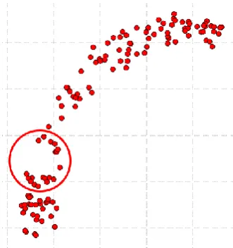
For more clarification, we will take the example of the two crescents as two separated clusters as shown in Figure 6. The issue appears when one of the crescents has low density region that causes the algorithm to break it into two clusters in addition to the existed crescent.

One of the solutions for this leak is by adjusting ε or minPts but this may cause another issue especially if clusters are close to each other enough to be merged as one cluster and this is not the required solution nor valid cluster (see Figure 7).

Figure 7: Two clusters and the result after applying density-based algorithms with invalid adjusting ε or minPts

Our proposed solution work after applying algorithm to expand the area of dense regions to link separated clusters as classified before. The process of expanding the area depends on selecting extra points that were already not selected as core or border when executing the algorithm. Selecting these points happens through selection models that were explained in section three of this paper.

The main idea of select model process is calculating the distance between unselected points and the clustered points. After calculation, the selection functions decide which points will be included in the closest cluster. The selected models which were tested gave us different results with the different arbitrary shapes of clusters. The best result was observed when applying F-measure quality model with density-based algorithm OPTICS. The next section discusses selecting statistical models with both density-based algorithms DBSCAN and OPTICS.

5.

EXPERIMINTAL RESULTS

In this paper, the selection and evaluation are applied by using laptop with Core2Duo processors under operating system windows.

The experimental implementation handles applying two clustering algorithms DBSCAN, and its extension OPTICS on 1850 artificial random sampling dataset and another dataset on the internet about schizophrenia disease divided into two clusters for male and female patients.

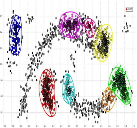
The random dataset created fitted many cases like high density and low, occasional and close points with arbitrary shape as presented in Figure 8.

As shown in Figure 8, region A presents an isolated cluster with small noise surrounding and a good distance away from other clusters, while region B contains three different clusters in

density and distance between each other. In addition, some noise causes the merge between upper and lower cluster when applying density-based algorithms with high ε. For region C, there are two clusters with good noise and good density, and the two dense regions are close enough to cause the merge between them after applying the algorithms.

Figure 8: Sample dataset contain 1850 random points

The evaluation is divided into two phases, DBSCAN with eps=0.06 and minPts=33

The selection of these two parameters depend on the density of points and is optimized many times to get better clustering for sample dataset generated in the current study. For all selection models, the best values for BIC, AIC, and RSS are low except F-measure score achieved the best result with high value.

Table 1: Number of clusters for each algorithms

Algorithm BIC AIC RSS

F-Measure

DBSCAN 6 8 7 6

OPTICS 7 6 7 4

Table 1 presents the actual result when applying the two clustering algorithms DBSCAN and OPTICS. Variant in results indicate good and useless results since the artificial already designed with four main clusters, and the close result comes from using OPTICS algorithm since it is the extended version of DBSCAN algorithm. Close result shaped after using F1 metric measurement as shown in Figure 8.

In Figure 9 clearly the result of applying DBSCAN produces 7 different clusters and a wide range of noise, so I continued with testing other selection models to improve the result of cluster size.

Figure 10: Applying DBSCAN with Euclidean distance and optimized by BIC

When applying BIC function, the observation result became negative since the number of clusters decreases and the noise points increase as shown clearly in Figure 10.

Figure 11: Applying OPTICS with Euclidean distance and optimized by AIC

When the algorithm changed to OPTICS with the same parameters ε = 0.06 and minPts=30, then the result was optimized using statistical models, the observation achieve better result in cluster number as appeared in Figure 11. But when applying more testing, the result of clustering get best cases with F-measure selection model and OPTICS algorithm

for both number of clusters and the selected point within each cluster as shown clearly in Figure 12.

Figure 12: Shows clustering dataset using OPTICS algorithm and optimized by F-measure selection model

The second dataset under this experiment was for a schizophrenia patient as shown in Figure 13. It is clear that the dataset, divided into two clusters, presents distribution of the disease based on gender and age.

Figure 13 : Gender and age of schizophrenia patient’s dataset

Therefore, the observation for the two clustering algorithms has a high error rate which results from the two clusters that contain variant density data.

Figure 14: Results of executing DBSCAN (top) and OPTICS (bottom)

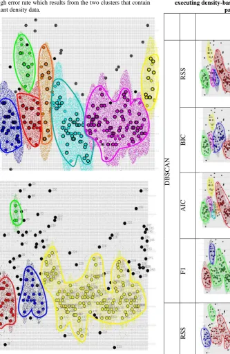
Table 2 below summarizes the applying of selection models after executing both of density-based algorithms DBSCAN and OPTICS. In addition, it compares the outcome with origin dataset that was already clustered to judge which selection model get better results after applying.

Table 2: Results of applying all selection models after executing density-based algorithms with schizophrenia

patients’ dataset.

# of clus ters

Description

DB

S

C

AN

R

SS 5

Enhancement of the number of clusters, but the error ratio is still high

B

IC 5

Same as with RSS, the updates

become in

selecting points.

AI

C 7

This model increases the

number of

clusters and this is not preferable.

F1

3

F-score result is better than the other algorithms as seen here.

OPTI

C

S

R

SS 3

With OPTICS, the result is more accurate and close to real clustered dataset.

B

IC 3

AI

C 3

The selection and enhancement become better and close enough to the required outcome.

F1

2

This result is the most accurate result to real clustered dataset

6.

CONCLUTION

This paper studies applying selection modeling to achieve better results for clustering dataset with density distribution.

The selection models that optimize the clustering method are BIC, AIC, RSS, and F1. These models already enhance the number of points within clustered dataset by DBSCAN or OPTICS algorithm.

The good results appear when applying the F-measure selection model as observed in Figures when the number of points within the cluster increased and noise points decreased.

For further future studies, applying these selection models and other statistical models on other Density-based clustering algorithms is recommended.

7.

REFERENCES

[1] Amin Karami , Ronnie Johansson “Choosing DBSCAN Parameters Automatically using Differential Evolution”, 2014.

[2] Krista Rizman, Zalik. An efficient “k-means clustering algorithm.Pattern Recognitoin Letters”, 2008.

[3] Martin Ester, Hans-Peter Kriegel, Jörg Sander, Xiaowei Xu, “A Density-based Algorithm for Discovering Clusters in Large Spatial Databases with Noise”, 1996.

[4] Mohammed T. H. Elbatta, and Wesam M. Ashour, “A Dynamic Method for Discovering Density Varied Clusters”,2013

[5] Manisha Naik Gaonkar & Kedar Sawant ,“AutoEpsDBSCAN : DBSCAN with Eps Automatic for Large Dataset”, 2013.

[6] Anne Denton, “Density-based Clustering of Time Series Subsequences”, 2005

[7] A. Hinneburg and D. Keim. “A general approach to clustering in large databases with noise”, 2003.

[8] Ankerst, M., Breunig, M., Kriegel, H.P., Sander, J. “OPTICS: Ordering Points To Identify the Clustering Structure”, 1999.

[9] Vladimir Spitalsky, Marian Grendar “OPTICS-based clustering of emails represented by quantitative profiles”, 2013.

[10]Walter Zucchini, “An Introduction to Model Selection”, 2000

[11]Hamparsum Bozdogan, “Akaike's Information Criterion and Recent Developments in Information Complexity”, 2000.

[12]Tsong Yueh Chen , Fei-Ching Kuo , Robert Merkel, “On the Statistical Properties of the F-measure” 2004.

[13]Abdolreza Rasouli, Mohd Aizaini Bin Maarof, Mahboubeh Shamsi, “A New Clustering Method Based on Weighted Kernel K-Means for Non-linear Data”, 2009.

[14]Nan Ye, Kian Ming A. Chai, Wee Sun Lee, Hai Leong Chieu, “Optimizing F-Measures: A Tale of Two Approaches”,2012

[15]Jörg Sander, Xuejie Qin, Zhiyong Lu, Nan Niu, Alex Kovarsky, “Automatic Extraction of Clusters from Hierarchical Clustering Representations”,2003

[16]Eric Yi Liu, Zhishan Guo, Xiang Zhang, Vladimir Jojic and Wei Wang, “Metric Learning From Relative Comparisons by Minimizing Squared Residual”,2012