Prediction of the Bombay Stock Exchange (BSE) Market
Returns Using Artificial Neural Network and Genetic
Algorithm
Yusuf Perwej1, Asif Perwej2
1Computer Science & Information System, Jazan University, Jazan, Kingdom of Saudi Arabia (KSA); 2Department of Management, Singhnia University, Rajasthan, India.
Email: {yusufperwej, asifperwej}@gmail.com
Received April 6th, 2011; revised February 6th, 2012; accepted February 13th, 2012
ABSTRACT
Stock Market is the market for security where organized issuance and trading of Stocks take place either through ex- change or over the counter in electronic or physical form. It plays an important role in canalizing capital from the in- vestors to the business houses, which consequently leads to the availability of funds for business expansion. In this pa- per, we investigate to predict the daily excess returns of Bombay Stock Exchange (BSE) indices over the respective Treasury bill rate returns. Initially, we prove that the excess return time series do not fluctuate randomly. We are apply- ing the prediction models of Autoregressive feed forward Artificial Neural Networks (ANN) to predict the excess return time series using lagged value. For the Artificial Neural Networks model using a Genetic Algorithm is constructed to choose the optimal topology. This paper examines the feasibility of the prediction task and provides evidence that the markets are not fluctuating randomly and finally, to apply the most suitable prediction model and measure their effi- ciency.
Keywords: Stock Market; Genetic Algorithm; Bombay Stock Exchange (BSE); Artificial Neural Network (ANN);
Prediction; Forecasting; Data; Autoregressive (AR)
1. Introduction
It is nowadays a common notion that vast amounts of capital are traded through the Stock Markets all around the world. National economies are strongly linked and heavily influenced by the performance of their Stock Markets. The characteristic that all Stock Markets have in common is the uncertainty, which is related with their short and long term future state. This feature is undesi- rable for the investor but it is also unavoidable whenever the Stock Market is selected as the investment tool. The best that one can do is to try to reduce this uncertainty. Stock Market Prediction (or Forecasting) is one instru- ment in this process.
The Stock Market prediction task divides researchers and academics into two groups those who believe that we can devise mechanisms to predict the market and those who believe that the market is efficient and whenever new information comes up the market absorbs it by cor- recting itself, thus there is no space for prediction. Fur- thermore they believe that the Stock Market follows a Random Walk, which infers that the best prediction you can have about tomorrow's value is today’s value.
2. Stock Market
A place, whether physical or electronic, where stocks in listed companies are bought and sold. A stock market may be a private company, a non-profit, or a publicly- traded company. A stock market provides a regulated place where brokers and companies may meet to make investments on neutral ground. The stocks are listed and traded on stock exchanges which are entities of a cor- poration or mutual organization specialized in the business of bringing buyers and sellers of the organizations to a listing of stocks and securities together. The stock market in the India is the Bombay Stock Exchange. Participants in the stock market range from small individual stock investors to large hedge fund traders, who can be based anywhere. Their orders usually end with a professional at a stock exchange, who executes the order.
man called Van der Beurze, and in 1309 they became the “Brugse Beurse”, institutionalizing what had been, until then, an informal meeting, but actually, the family Van der Beurze had a building in [1] Antwerp where those gatherings occurred, the Van der Beurze had Antwerp, as most of the merchants of that period, as their primary place for trading. The idea quickly spread around Flanders and neighboring counties and “Beurzen” soon opened in Ghent and Amsterdam.
In the middle of the 13th century, Venetian bankers began to trade in government securities. In 1351 the Ve- netian government outlawed spreading rumors intended to lower the price of government funds. Bankers in Pisa, Verona, Genoa and Florence also began trading in govern- ment securities during the 14th century. This was only possible because these were independent city states not ruled by a duke but a council of influential citizens. The Dutch later started joint stock companies, which let share- holders invest in business ventures and get a share of their profits or losses. In 1602, the Dutch East India Com- pany issued the first share on the Amsterdam Stock Ex- change. It was the first company to issue stocks and bonds.
2.1. Investment Theory
An investment theory suggests what parameters one should take into account before placing his (or her) ca- pital on the market. Traditionally the investment commu- nity accepts two major theories 1st the Firm Foundation and 2nd the Castles in the Air [2]. These theories allow us to understand how the market is shaped, or in other words how the investors think and react. It is this se-quence of “thought and reaction” by the investors that define the capital allocation and thus the level of the market. There is no doubt that most of the people related to stock markets are trying to achieve profit. Profit comes from investing in stocks that have a good future. What they are trying to accomplish one way or the other is to predict the future of the market. But what determines this future? The way that people invest their money is the answer and people invest money based on the informa-tion they hold. Therefore we have the following schema in Figure 1.
[image:2.595.309.537.87.123.2]The factors that are under discussion on this schema is
Figure 1, the content of the “Information” component
and the way that the “Investor” reacts when having this information. According to the Firm Foundation theory the market is defined from the reaction of the investors, which is triggered by information that is related to the “real value” of firms. The “real value” or else the intrin- sic value is determined by careful analysis of present conditions and future prospects of a firm [3]. On the oth-er hand, according to the Castles in the Air theory the investors are triggered by information that is related to other investor’s behavior. So for this theory the only concern that
Figure 1. Investment procedure.
the investor should have is to buy today with the price of 20 and sell tomorrow with the price of 30, no matter what the intrinsic value of the firm he (or she) invests in is. Therefore the Firm Foundation theory favors the view that the market is defined mostly by logic, while the Ca- stles in the Air theory supports that the market is defined mostly by psychology.
2.2. Data Related to the Market
The information about the market comes from the study of the relevant data. Here we are trying to describe and group into categories the data that relate to the stock markets. In this paper these data are divided into three major categories [4].
Technical data: This type of all the data that refer to stocks only. Technical data include:
■ The price at the end of the day.
■ The highest and the lowest price of a trading day. ■ The volume of shares traded per day.
Fundamental data: This type of data related to the intrinsic value of a company or category of com- pa-nies as well as data related to the general economy. Fundamental data include:
■ Inflation. ■ Interest Rates. ■ Trade Balance.
■ Indexes of industries (e.g. Heavy industry). ■ Net profit margin of a firm.
■ Prognoses of future profits of a firm.
Derived data: This type of data can be produced by transforming and combining technical and/or funda- mental data. Some commonly used examples are:
Returns: This type of One-step returns R(t) is defined
as the relative increase in price from the previous point in a time series. Thus if y(t) is the value of a
stock.
On day t,
1 ( )
1 y t y t R t
y t
Volatility: This type of Describes the variability of a stock and is used as a way to measure the risk of an investment.
3. Prediction of the Market
3.1. Defining the Prediction Task
Before having any further discussion about the prediction of the market we define the task in a formal way. “Given a sample of N examples {(xi, yi), I = 1,…, N} where f(xi)
= yi, i, return a function g that approximates f in the
sense that the norm of the error vector E = (e1,…, eN) is
minimized. Each ei is defined as ei = e(g(xi), yi) where e
is an arbitrary error function”. In other words the defini-tion above shows that to predict the market you should search historic data and find relationships among these data and the value of the market. Then try to exploit these relationships you have found in future situations. This defi- nition is based on the assumption that such relationships do exist. But do they? Or do the markets fluctuate in a totally random way leaving us no space for prediction? This is a question that has to be answered before any attempt for prediction is made.
3.2. Prediction Method
The prediction of the market is without doubt an inte- resting task. In the literature there are several methods applied to accomplish this task. These methods use va- rious approaches, ranging from highly informal ways (e.g. the study of a chart with the Fluctuation of the market) in more formal ways (e.g. Linear or non-linear regressions). We have categorized these techniques as follows:
Traditional Time Series Prediction Methods;
Machine Learning Methods.
The criterion to this categorization is the type of tools and the type of data that each method is used to predict the market. What is common to these techniques are that they are used to predict and thus benefit from the mar- ket’s future behavior. None of them has proved to be the consistently correct prediction tool that the investor would like to have. Furthermore many analysts question the usefulness of many of these predictions techniques.
3.2.1. Traditional Time Series Prediction
The Traditional Time Series Prediction analyzes historic data and attempts to approximate future values of a time series as a linear combination of these historical data. In econometrics there are two basic types of time series forecasting: univariate (simple regression) and multiva- riate (multivariate regression) [6]. These types of regres- sion models are the most common tools used in econo- metrics to predict time series. The way they are applied in practice is that first a set of factors that influence (or more specific is presumed that influence) the series under prediction is formed. These factors are the explanatory variables xi of the prediction model. Then a mapping
between their values xit and the values of the time series
yt (y is the to-be explained variable) is done, so that pairs
{xit, yt} are formed. These pairs are used to define the
importance of each explanatory variable in the formula-tion of the explained variable. In other words the linear combination of xi that approximates in an optimum way y is defined. Univariate models are based on one ex-planatory variable (I = 1) while multivariate models use more than one variable (I > 1). Regression models have been used to predict stock market time series. A good example of the use of multivariate regression is the work of Pesaran and Timmermann (1994) [7].
3.2.2. Machine Learning Method
Machine learning is a process that begins with the iden- tification of the learning domain and ends with testing and using the results of the learning. It will be useful to start with an overview of how a machine learning system is developed, trained, and tested. The key parts of this process is the “learning domain,” the “training set,” the “learning system,” and “testing” the results of the learn- ing process [8]. All these methods use a set of samples to generate an approximation of the underlying function that generated the data. The aim is to draw conclusions from these samples in such a way that when unseen data are presented to a model it is possible to infer the to be explained variable from these data. The methods we dis- cuss here are the [9] Neural Networks Techniques. These methods have been applied to market prediction particu- larly for Artificial Neural Networks there is a rich litera- ture related to the forecast of the market on a daily basis.
4. Bombay Stock Exchange (BSE)
talization-weighted methodology is a widely followed index construction methodology on which majority of global equity indices are based; all major index providers like MSCI, FTSE, STOXX, S&P and Dow Jones uses the free float methodology.
5. Artificial Neural Network
The artificial neural network is simplified models of the biological neuron system, is a massively parallel distri- buted processing system made up of highly intercon-nected neural computing elements that can learn and thereby acquire knowledge and make it available for use. The artificial neural network learns by example. They can therefore be trained with known examples of a prob-lem to acquire knowledge about it. Once appropriately trained, the network can be put to effective use in solving unknown or untrained instances of the problem.
5.1. Neuron
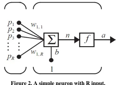
A neuron is a processing unit that takes several inputs and gives a distinct output. The Figure 2 below depicts
a single neuron with R inputs p1, p2,…, pR, each input
is weighted with a value w11, wl2,…, wlR and the output
of the neuron an equal to f (w11·p1 + w12·p2 +…+ w1R·pR).
Each neuron apart from the number of its input is cha-racterized by the function f known as a transfer func- tion. The most commonly used transfer functions are the hard-limit, the purelinear, the sigmoid and the tansigmoid function Table 1 shows. The preferences on these func-
tions derive from their characteristics. Hardlimit maps any value that belongs with
,
into two distinct values {0, 1}, thus it is preferred for networks that per- form classification tasks (multiplayer perceptrons MLP). Sigmoid and tansigmoid, known as squashing functions, map any value from to the intervals [0, 1] and [–1, 1] respectively. Lastly purelinear is used due to its ability to return any real value and is mostly used at the neurons that are related to the output of the network in Table 1.
, [image:4.595.329.517.86.224.2]5.2. Layer
Figure 3 presents the Artificial Neural network is de-
fined as data processing system consisting of many of simple highly interconnected processing elements (artifi- cial neurons) is an architecture inspired by the structure of the cerebral cortex of the brain. Each network has got exactly one input layer, zero or more hidden layers and one output layer. All of them apart from the input layer consist of neuron. The number of inputs to the Artificial Neural Networks equal to the dimension of our input samples Figure 3 shows, while the number of the outputs
we want from the Artificial Neural Networksdefine the number of neurons in the output layer. In our case the
Figure 2. A simple neuron with R input.
Table 1. The most commonly used transfer function.
Hardlimit Purelinear Sigmoid Tansigmoid
1, 0 ( )
0, 0 x f x
x
f x( )x
1 ( )
1 x f x
e
2
2
( ) 1
1 n
f x e
[image:4.595.305.540.249.493.2]
( ) {0,1}
f x f x( ) ( , ) f x( ) [0,1] f x( ) [ 1,1]
Figure 3. Neural Network Diagram.
output layer will have exactly one neuron since the only output we want from the network is the prediction of tomorrow’s excess return.
The mass of hidden layers as well as the mass of neu- rons in each hidden layer is proportional to the ability of the network to approximate more complicated functions. Of course this does not infer by any means that networks with complicated structures will always perform better. The reason for this is that the more complicated a net- work is the more sensitive it becomes to noise or else, it is easier to learn apart from the underlying function the noise that exists in the input data. Therefore clearly there is a trade off between the representational power of a net- work and the noise it will incorporate.
5.3. Weight
ficial Neural Networks and the characterization of a net- work. The procedure of adjusting the weights of a Artifi- cial Neural Networks based on a specific dataset is re- ferred as the training of the network on that set (training set). The basic idea behind training is that the network will be adjusted in a way that will be able to learn the patterns that lie in the training set. Using the adjusted network in future situations (unseen data) it will be able based on the patterns that learned to generalize giving us the ability to make inferences. In our case we will train the Artificial Neural Network model on a part of our time series (training set) and we will measure their ability to generalize on the remainning part (test set). The size of the test set is usually selected to be 10% of the available samples [11]. Each sample consists of two parts the input and the target path is called supervised learning. Initially the weights of the network is assigned random values (usually within [–1, 1]). Then the input part of the first sample is presented to the network. The network com- putes an output based on: the values of its weights, the number of its layers and the type and mass of neurons per layer.
There are two major categories of network training the incremental and the batch training. During the incre- mental training the weights of the network is adjusted each time that each one of the input samples are pre- sented to the network, while in batch mode training the weights are adjusted only when all the training samples have been presented to the network.
5.4. Training Algorithm
The mechanisms of weights update are known as training algorithm. The algorithms described here are related to feed-forward networks. Artificial Neural Networks are characterized as feed-forward network if it is possible to attach successive numbers of the inputs and to all the hidden and output units such that each unit only receives connections from inputs or units having a smaller num- ber [12]. All these algorithms use the gradient of the cost function to determine how to adjust the weights to mini- mize the cost function. The gradient is determined using a technique called backpropagation, which involves perform- ing computations backwards through the network.
5.5. Gradient Descent
We will describe in detail the way that the weights of a feed forward network are updated using the backpropa- gation gradient descent algorithm. The following des- cription is related to the incremental training mode. We introduce the notion we will use.
If EN
w
is the value of the error function of the sample
N and the vector with all the weights of the network then the gradient of EN in respect to w is
11 12
, , ,
N N N
N
mn
E E E
E w
w w w
Where jiis the weight that is related with the neuron j
and its input i. “When interpreted as a vector in weight
space, the gradient specifies the direction that produces the steepest increase in
w
N
E .The negative of this vector
therefore gives the direction of the steepest decrease”. Based on this concept we are trying to update the weights of the network according to
'
w w Aw
( )
N
Aw E w
Here is a positive constant called the learning rate, the greater is the greater the change in . w
ji
x , is the i-th input of unit j, presuming that each
neuron is assigns a number successively.
ji
w , the weight associated with the i-th input to neuron j.
j
iw xji jinet (The weighted sum of inputs of neu-
ron j)
j
á , the output computed by node j.
j
t , the target of output unit j.
ó, the sigmoid function.
Outputs, the set of nodes in the final layer of the net- work.
Downstream (j), the set of neurons whose immediate
inputs include the output of neuron j.
If we make the assumption that we have a network with neurons that use the sigmoid transfer function (ó) then we will try to calculate the gradient EN wji
using the chain rule we have that
j
N N N
ji
ji j ji j
net
E E E
x
w net w net
5.6. Parameter Setting
The properties related to a neuron is the transfer function it uses as well as the way it processes its inputs before feeding them to the transfer function. The Artificial Neural Networks we will create use neurons that preprocess the input data as follow, If x1,…, xN are the inputs to the
neuron and w1,…, wN their weights the value fed to the
transfer function would be iN1 i i
x w
The neurons in the output layer will use the purelinear function while the neurons in the hidden layer the tan- sigmoid function. We select the tansigmoid and not the sigmoid since the excess return time series contains values in [–1, 1], thus the representational abilities of a tansig-moid function fit in a better way the series we attempt to predict comparable to those of the sigmoid’s. We will be following structure in Artificial Neural Networks x-y-z-1
where x, y can be any integer greater than one, while z
hidden layers the properties of their nodes. What remains open is the number of hidden units per layer as well as the number of inputs. Since there is no rational way of selecting one structure and neglecting the others we will use a search algorithm to help us to choose the optimum number of units per layer. The algorithm we will use is a Genetic Algorithm (GA). The Genetic Algorithms will search a part of the space defined by x-y-z-1 and will
converge towards the network structures that perform better on our task.
6. Genetic Algorithm
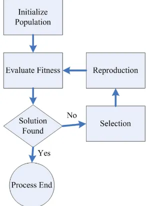
Genetic Algorithm proposed in 1975 by Johan Holland. Genetic Algorithms are computerized search and opti- mization algorithms based on the mechanics of natural genetics and natural selection. Genetic algorithms per- formed directed random searches through a given set of alternative with the aim of finding the best alternative with respect to the given criteria of goodness as illus- trated in Figure 4. The criteria are required to be ex-
pressed in terms of an objective function which is usually called a fitness function. Fitness is defined as a figure of merit, which is to be either maximized or minimized.
The biological organism to be specified is defined by one or by a set of chromosomes. The overall set of chro- mosomes is called genotype, and the resulting organism is called the phenotype. Every chromosome consists of genes. The gene position within the chromosome refers to the type of organism characteristic, and the coded content of each gene refers to an attribute within the organism type. In Genetic Algorithms terminology, the set of strings (chromosomes) forms a structure (geno- type). Each string consists of characters (genes). Genetic Algorithms are a method for moving from one popula- tion of “chromosomes” [13] (strings of 1, 0 bits) to a new population by using a kind of “natural selection” together with the genetics inspired operators of crossover, muta- tion, and inversion. Each chromosome consists of “genes” (bits), each gene being an instance of a particular “allele” (0 or 1). The selection operator chooses those chromo- somes in the population that will be allowed to reproduce, and on average the fitter chromosomes produce more offspring than the less fit ones. Crossover exchanges sub- parts of two chromosomes, roughly mimicking bio- log-ical recombination among two single chromosomes (haploid) organisms; mutation randomly changes the allele values of some locations in the chromosome; and the inversion reverses the order of a contiguous section of the chromosome, thus rearranging the order in which genes are arrayed.
6.1. A Conventional Genetic Algorithm
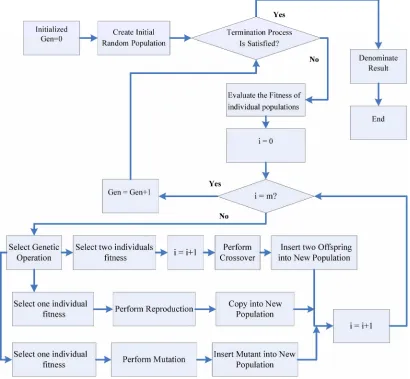
[image:6.595.349.495.86.292.2]A genetic algorithm has the three major components. The
Figure 4. Flow chart of genetic algorithm iteration.
first component is related to the creation of an initial population of m randomly selected individuals. The ini- tial population shapes the first generation. The second component inputs m individuals and gives as output an evaluation for each of them based on an objective func- tion has known as fitness function shown in Figure 5.
This evaluation describes how close to our demands each one of these m individuals is and the third component is responsible for the formulation of the next generation. A new generation is formed based on the fittest individuals of the previous one. This procedure of evaluation of ge- neration N and production of generation N + 1 (based on N) is iterated until a performance criterion is met. The creation of offspring based on the fittest individuals of the previous generation is known as breeding. The breeding procedure includes three basic genetic operation reproduction, crossover and mutation.
Reproduction selects probabilistically one of the fittest individual of generation N and passes it to generation N + 1 without applying any changes to it. On the other hand, crossover selects probabilistically two of fittest indivi- duals of generation N then in a random way chooses several their characteristics and exchanges them in a way that the chosen characteristics of the first individual would be obtained by the second a vice versa as illus-trated in Figure 5. Following this procedure creates two
new offspring that both belong with the new generation. Finally the mutation selects probabilistically one fittest individual and changes several its characteristics in a random way showed in Figure 5. The offspring that
Figure 5. A conventional Genetic Algorithm.
It is clear from the flowchart of the Genetic Algo- rithms that each member of a new generation comes ei- ther from a reproduction, crossover or mutation operation. The operation that will be applied each time is selected based on a probabilistic schema. Each one three opera- tions is related to a probability Preproduction, Pcrossover, and Pmutation in a way that
Preproduction + Pcrossover + Pmutation = 1
Therefore the number of offspring that comes from re- production, crossover or mutation is proportional to Pre- production, Pcrossover, and Pmutation respectively [15].
6.2. A Genetic Algorithm That Define the Artificial Neural Network Structure
We use Genetic Algorithms to search a space of Artifi- cial Neural Network topologies and select those that match optimally our criteria. The topologies that interest us have at most two hidden layers and their output layer has the one neuron (x-y-z-1). Due to computational limi-
tations it is not possible search the full space defined by
x-y-z-1. What we can do is to search the space defined by xmax-ymax-zmax-1, where xmax, ymax and zmax are upper limits
we set for x, y and z respectively.
7. Proposed Prediction Using Artificial
Neural Network
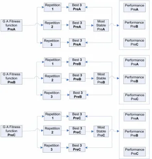
The proposed prediction consisted of three phases Figure 6. In the first phase a Genetic algorithm searched the
space of Artificial Neural Networks with different struc- tures and resulted a generation with the fittest of all net- works searched based on a metric which was either PreA or PreB or PreC [16]. The Genetic Algorithms search was repeated three times for each metric. Then the best three networks were selected from each repetition of the Genetic Algorithms search and for each one metrics. The output of the first phase was a set of thirty six network structures shown in Figure 6.
Figure 6. Experiment of BSE Data.
used the showed number of epochs from the validation procedure and based on it we retrained the network on the Training1 plus the Validation 1 set. Finally we tested the performance of the network for unseen data (Valida- tion 2 set). This procedure was repeated 50 times for each network structure for random initializations of its weights. From the nine networks for each performance statistic, we selected the most stable in terms of standard deviation of their performance. Thus the output of the second phase was a set of four network structures. Dur-ing the third phase for each one of these four networks we applied the following procedure 50 times. We trained each network on the first half of the Training Set and we used the remaining half for validation. Then, using the showed epochs by the validation procedure, we retrained the network on the complete Training Set as illustrated in
Figure 6. Finally we tested the network on the Test Set
calculating all four metrics. The performance for each network on each metric was measured again in terms of standard deviation and mean of its performance over 50 times that it was trained, [17] validated and tested.
In this paper first set of parameters is related to the size of the space that the Genetic Algorithm will search. We constructed this is set through variables xmax, ymax and
zmax which represent the size of the input, the first
hidden and the second hidden layer respectively. For all the Genetic Algorithms in this study we have used xmax =
30, ymax = 40 and zmax = 40. This decision was made hav-
ing in mind that the larger the space the smaller the probability of neglecting network structures that might perform well in our task. We have selected the larger space that we could search keeping in mind our compu- tational constraints. All the experiments proved that the most interesting part of our search space was not close to these bounds therefore we concluded that the search space needed no expansion. We observed that the Resi- lient Backpropagation is the algorithm that converged fastest and in fewest epochs. Our observations on the performances of these algorithms agree with the observa- tions of Demuth and Beale [18]. They also experimented on specific network structures using different data and they found that the Resilient Backpropagation converges faster than all the other algorithms we considered in our research.
8. Experimental Results of Bombay Stock
Exchange (BSE)
of our metrics (PreA, PreB, PreC).
PreA
By evaluating the networks based on PreA the Genetic algorithm search for the first repetition gave us the fol- lowing results. The first two columns of shown in Table 2 describe the initial generation that contains 30 ran-
domly selected networks and their performance (PreA), while the next two columns give the individuals [19] of the last generation with their performance. The ten net- work structures that were mostly visited by the algorithm as well as the frequency with which they were met in the 25th generation are shown by the following Table 2.
We have that the network with structure 6-19-3-1 was considered by the algorithm 61 times and it was not pre- sent in the final generation, while network 11-6-3-1 was considered 50 times and it was met 9 times in the 25th generation. Table 2 shows that the variance of the per-
formance of the networks in Generation 1 is small and their average is close [20] to one. The performance of the networks belongs to the last generation shows that most of them performed only as well as the random walk model based on the price of the market. This can be ei- ther because there are no structures that give significantly better results compared to the random walk model or that the path that our algorithm followed did not manage to discover these networks. Therefore, to have safer conclu- sions we selected to repeat the search twice. A second comment is that there are network structures that seem to perform very badly, for instance 10-29-21-1 gave us PreA of 4.5. Furthermore from Table 2 it is clear that the
Genetic Algorithms did manage to converge to network with smaller in both terms of mean and standard devia- tion. The type of network structures we got in the final generation the only pattern we observed was a small second hidden layer and more Specifically 3 neurons for most of our structures. How fit individuals proved to be throughout the search that the algorithm performed. For instance the network 6-19-3-1 was visited 60 times, which infers that for a specific time period this individual managed to survive but a farther search of the algorithm proved that new fittest individuals came up and 6-19-3-1 did not manage to have a place at the 25th generation. The next step we repeated the Genetic Algorithms search. The results we obtained in terms of the mean and stan- dard deviation of the first and last generations were
Repetition 3
Generation first last
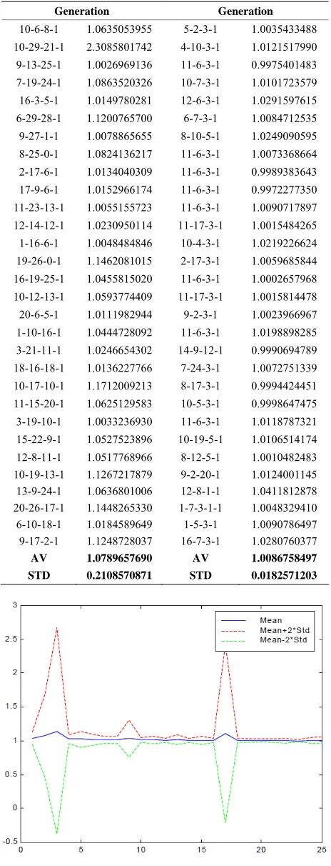
Average 1.031067456 0.017527960 Std 0.043528247 0.023318392 The simulation results shown in Figure 7 were gene-
[image:9.595.309.538.97.713.2]rated with Matlab following plots give the mean and the standard deviation of PreA for each generation (from 1 to 25). In addition the overall generations mean and stan-dard deviation is reported.
Table 2. The results of the First Repetition of the Genetic Algorithms search on the Bombay Stock Exchange data.
Generation Generation
10-6-8-1 1.0635053955 5-2-3-1 1.0035433488 10-29-21-1 2.3085801742 4-10-3-1 1.0121517990
9-13-25-1 1.0026969136 11-6-3-1 0.9975401483 7-19-24-1 1.0863520326 10-7-3-1 1.0101723579 16-3-5-1 1.0149780281 12-6-3-1 1.0291597615 6-29-28-1 1.1200765700 6-7-3-1 1.0084712535
9-27-1-1 1.0078865655 8-10-5-1 1.0249090595 8-25-0-1 1.0824136217 11-6-3-1 1.0073368664 2-17-6-1 1.0134040309 11-6-3-1 0.9989383643 17-9-6-1 1.0152966174 11-6-3-1 0.9972277350 11-23-13-1 1.0055155723 11-6-3-1 1.0090717897 12-14-12-1 1.0230950114 11-17-3-1 1.0015484265 1-16-6-1 1.0048484846 10-4-3-1 1.0219226624 19-26-0-1 1.1462081015 2-17-3-1 1.0059685844 16-19-25-1 1.0455815020 11-6-3-1 1.0002657968 10-12-13-1 1.0593774409 11-17-3-1 1.0015814478 20-6-5-1 1.0111982944 9-2-3-1 1.0023966967 1-10-16-1 1.0444728092 11-6-3-1 1.0198898285 3-21-11-1 1.0246654302 14-9-12-1 0.9990694789 18-16-18-1 1.0136227766 7-24-3-1 1.0072751339 10-17-10-1 1.1712009213 8-17-3-1 0.9994424451 11-15-20-1 1.0625129583 10-5-3-1 0.9998647475 3-19-10-1 1.0033236930 11-6-3-1 1.0118787321 15-22-9-1 1.0527523896 10-19-5-1 1.0106514174 12-8-11-1 1.0517768966 8-12-5-1 1.0010482483 10-19-13-1 1.1267217879 9-2-20-1 1.0124001145
13-9-24-1 1.0636801006 12-8-1-1 1.0411812878 20-26-17-1 1.1448265330 1-7-3-1-1 1.0048329410
6-10-18-1 1.0184589649 1-5-3-1 1.0090786497 9-17-2-1 1.1248728037 16-7-3-1 1.0280760377
AV 1.0789657690 AV 1.0086758497 STD 0.2108570871 STD 0.0182571203
[image:9.595.308.540.111.717.2]Repetition 3
Repetition 3 Minimum 0.9795799885 Maximum 5.3546777648 Mean 1.0365190398 StDev 0.1147578350 The above plots make clear that in all repetitions the Genetic Algorithms converged giving us networks with smaller Pres. It is also clear that the standard deviation of the Pres across generations also converted to smaller va- lues. However in none of these experiments did we ob- tain a network structure that clearly beats the random walk model shown in Figure 7. Furthermore the patterns
we managed to observe in the topologies of the networks that belong with the last generations are first, topologies with many neurons in both hidden layers and in the input layer were not prepared and secondly, the fittest networks proved to be those with one or three neurons in the second hidden layer. The most occurrences that a specific topology managed to have in a last generation were 9, we disco- vered no network that was by far better than all the others.
PreB
Similarly, we used the Genetic Algorithms to search the space of network topologies using PreB As fitness function. The means and standard deviations of the first and last generation forall repetitions are presented in the following.
Repetition 2
Generation First Last
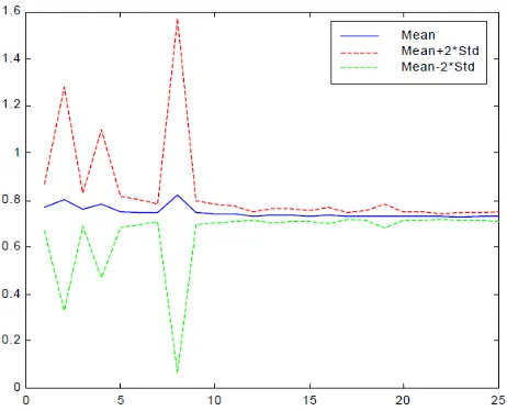
Average 0.760946598 0.716306695 Std 0.053750167 0.015607519 These results show that the Artificial Neural Network model managed to beat clearly the predictions of the RW model (based on the excess returns) by achieving on ave- rage Pres close to 0.69. A second important comment is that the Genetic Algorithms converged significantly both in terms of mean and standard deviation. While for PreA the average performance in both the first and the last generations was close to one and the only thing that the algorithm managed to achieve was to reduce the variance of the performance, for PreB we observed a significant im- provement not only to the variance but to the average of the performance as well. Furthermore in the first repeti- tion of the Genetic Algorithms search we obtained a to- pology that proved to be clearly the fittest; it was present 28 times in the last generation and it was visited by the Genetic Algorithms 243 times. The topology was 6-6-1-1.
The mean and standard deviation we obtained for each generation in each one three repetition are depicted by the shown in Figure 8.
Repetition 2
[image:10.595.307.538.84.271.2]Repetition 2 Minimum 0.7234528054 Maximum 3.1217654038 Mean 0.7544526178 StDev 0.0973071734
Figure 8. Mean and STD of PreB throughout all generation for the Bombay Stock Exchange data.
From these plots clearly the Genetic Algorithms con- verged in all repetitions both in terms of standard devia- tion and mean. This convergence was not always stable shown in Figure 8.
PreC
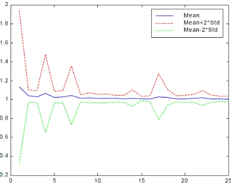
The Genetic Algorithms search using as fitness func- tion PreC gave us again values close to one shown in
Figure 9. Thushere it is shown that the Artificial Neural
Network model did not manage to beat clearly themodel which states that the gains we will have from the stock market is exactly thosethat we would have from bonds.
Repetition 3
Generation first Last
Average 1.175302645 1.005318149 Std 0.431630851 0.017530157 Here again in repetitions 3 we heard that the fittest network topologies had a second hidden layer that con- sisted of one or two nodes. The mean and standard de- viation throughout the 25 generations converted to small- ler values but repetitions 3 they moved asymptotically close to one; similarly to the case we used as fitness function the PreA.
Repetition 3
Repetition 3 Minimum 0.9785128058 Maximum 3.2870893626 Mean 1.0264347153 StDev 0.1078208731 From all the repetitions of the Genetic Algorithms search using both PreA and PreC itbecame clear that the predictive power of predictive models that are involved is similarly shown in Figure 9.
Figure 9. Mean and STD of PreC throughout all generation for the Bombay Stock Exchange data.
model which states that the value of the market tomorrow will be such that will allow us to have the same benefit from the stock market as we would have from the bond market (PreC). The benchmark that compares the Artifi- cial Neural Network model with the random walk model on the excess returnsturned out to be easy to beat always. Furthermore according to all the benchmarks that in- volved PreA or PreC there are naive prediction models that can perform equally well with the best Neural Net- works thus the Artificial Neural Networks did not man- age to outperform the predictive power of these models. The comment we must make here about PreA, B and C is that the naïve predictors related with PreA and PreC compare the predictive abilities of our models with naïve models that show no change in the value of the Bombay Stock Exchange market.
However we cannot say the same for the naïve predic- tor we use in PreB this predictor attempt to give us a pre- diction other that no change in the value of the Bombay Stock Exchange market. Therefore the naive predictors that are based on the statement that will be no change to the value of the market seems to be the most difficult to beat. The exhaustive search we performed in the experi- ment we have no doubt as to weather their might be a network topology for which the Neural Networks will be able to give better predictions. The search we have shown that there is no specific network structure that performs significantly better than the others, instead of there is a group of structures that gave us optimal per- formance, even though this performance is no betterthan that provided by a random walk.
9. Conclusion
Finally, the Artificial Neural Network model is superior compared to the Autoregressive models because they are
able to capture not only linear but also non linear patterns in the underlying data but their performance is influenced by the way that their weights are initialized. Therefore the evaluation of Artificial Neural Network model should be done not in terms of any one specific initialization of their weights, but in terms of the mean and standard de-viation of several randomly selected initializations. In the current study predicted of the Bombay Stock Exchange Market excess returns on a daily basis was attempted. More specifically we attempted to predict the excess re-turns of Bombay Stock Exchange (BSE) Stock Market the time series data of stock prices was transformed into the returns the investor would have if he selected the Stock Market instead of placing his capital in the bond market (excess return time series). In our prediction task we used lagged values of the excess return time series to predict the excess returns of the market on a daily basis. We applied randomness tests on the excess return time series the run and the test and we rejected randomness. Thus, we proved that the prediction task is feasible. Ro-bustness of Artificial Neural Networks to the changing structures, it can easily manage the inaccuracy and any degree of nonlinearity in the data.
REFERENCES
[1] O. B. Antwerpen, “6de Eeuwse Traditionele Bak- en Zan- dsteenarchitectuur,” 2010.
http://www.belgiumview.com/belgiumview/tl1/view0002 205.php4
[2] B. G. Malkei, “A Random Walk Down Wall Street,” 7th Edition, W. W. Norton & Company, New York, 1999. [3] R. Gupta., “Emerging Markets Diversification: Are
Cor-relations Changing over Time?” International Academy of Business and Public Administration Disciplines (IABPAD) Conference, Orlando, 3-6 January 2006, pp. 331-351. [4] T. Hellstrom and K. Holmstrom, “Predictable Pattern in
the Stock Return,” 1998.
http://www.wbiconpro.com/2.Sandip.pdf
[5] P. Dennis, “Stock Splits and Liquidity: The Case of the Nasdaq-100 Index Tracking Stock,” Financial Review, Vol. 38, No. 3, 2003, pp. 415-433.
[6] G. S. Maddala, “Introduction to Econometrics,” 1st Edi- tion, Macmillan Publishing Company, New York, 1992. [7] H. M. Pesaran and A. Timmermann, “Forecasting Stock
Returns: An Examination of Stock Market Trading in the Presence of Transaction Costs,” Journal of Forecasting, Vol. 13, No. 4, 1994, pp. 335-367.
doi:10.1002/for.3980130402
[8] R. S. Michalski and G. Tecuci, “Machine Learning: A Multistrategy Approach,” Morgan Kaufmann, Waitham, 1994.
[9] E. Alpaydın, “Introduction to Machine Learning (Adap- tive Computation and Machine Learning),” MIT Press, Cambridge, 2004.
Economy,” 2001. http://www.rbi.org.in
[11] M. T. Mitchell, “Machine Learning,” 1st Edition, The McGraw-Hill Companies, New York, 1997.
[12] M. C. Bishop, “Neural Networks for Pattern Recogni- tion,” Oxford University Press, New York, 1996.
[13] E. D. Goldberg, “Genetic Algorithm in Search, Optimiza-tion, and Machine Learning,” Addison-Wesley, New York, 1989.
[14] M. T. Mitchell, “An Introduction to Genetic Algorithms,” MIT Press, Cambridge, 1997.
[15] R. J. Koza, “Genetic Programming on the Programming of Computers by Means of Natural Selection,” MIT Press, Cambridge, 1992.
[16] P. Healy, J. Ledyard, S. Linardi and R. J. Lowery, “Pre- diction Markets: Alternative Mechanisms for Complex Environments with Few Traders,” Management Science, Vol. 56, No. 11, 2010, pp. 1977-1996.
doi:10.1287/mnsc.1100.1226
[17] H. White, “Economic Prediction Using Neural Networks: The Case of IBM Daily Stock Returns,” Proceedings of the 2nd Annual IEEE Conference on Neural Networks, San Diego, 24-27 July 1988, pp. 451-458.
doi:10.1109/ICNN.1988.23959
[18] H. Demuth and M. Beale, “Neural Network Toolbox: For Use with Matlab,” 4th Edition, The MathWorks Inc., Na-tick, 1997.
[19] O. Castillo and P. Melin, “Simulation and Forecasting Complex Financial Time Series Using Neural Networks and Fuzzy Logic,” IEEE International Conference on Systems, Man, and Cybernetics, Tucson, 7-10 October 2001, pp. 2664-2669.