Identifying the determinants and spatial nexus of provincial carbon intensity in China: A dynamic spatial panel approach

Munich Personal RePEc Archive

Identifying the determinants and spatial

nexus of provincial carbon intensity in

China: A dynamic spatial panel approach

Zheng, Xinye and Yu, Yihua and Wang, Jing and Deng,

Huihui

Renmin University of China, Renmin University of China,

Chongqing Technology and Business University, University of

International Business and Economics

2013

Identifying the determinants and spatial nexus of provincial carbon

intensity in China: A dynamic spatial panel approach

Xinye Zheng School of Economics Renmin University of China

Beijing 100872, China [email protected]

Yihua Yu ()

School of Economics Renmin University of China

Beijing 100872, China [email protected]

Jing Wang School of Economics

Chongqing Technology and Business University Chongqing, 400067, China

[email protected]

Huihui Deng

Institute of International Economy

University of International Business and Economics Beijing 100029, China

[email protected]

Abstract Is emission intensity of carbon dioxide (CO2) spatially correlated? What determines the CO2

intensity at a provincial level? More importantly, what climate and economic policy decisions should

the China’s central and local governments make to reduce the CO2 intensity and prevent the

environmental pollution given that China has been the largest emitter of CO2? We aim to address

these questions in this study by applying a dynamic spatial system-GMM (generalized method of

moment) technique. Our analysis suggests that provinces are influenced by their neighbours. In

addition, CO2 intensities are relatively higher in the western and middle areas, and that the spatial

agglomeration effect of the provincial CO2 intensity is obvious. Our analysis also shows that CO2

intensity is nonlinearly related to GDP (gross domestic product), positively associated with

secondary-sector share and FDI (foreign direct investment), and negatively associated with population size.

Important policy implications are drawn on reducing carbon intensity.

1 Introduction

Economists, ecologists, private industries and government decision-makers have long been interested

in the relationship between economic growth and environmental quality (Burnett and Bergstrom,

2010). China has experienced a consistent and rapid economic growth since the economic reforms

started in 1978. However, the pressure from energy constraints and environmental pollution has been

increasingly serious over the same time period. In recent years, scholars have extended the study of

pollutants from the regular pollutants (say, sulphur dioxide (SO2), nitrogen dioxide (NO2), carbon

monoxide (CO), and particulate matters) to carbon dioxide (CO2), which has become the main driving

force of global climate changes. Especially, the increased demand for energy in China has generated

concomitant increase of carbon emissions, mainly measured by CO2 emissions in this study, which

poses an unprecedented challenge to China’s, and even global, environment and sustainable

development (Liu et al., 2010). China has been one of bigger contributors to the rapid growth of global

CO2 emissions, accounting for 44% of the increase in global CO2 emissions in 1990-2004 (Kahrl and

David, 2006). In 2007, the CO2 emissions ratio in China (defined as the total CO2 emissions of China

to that of the world) hit the historical highest level of 21.01% and simultaneously, China surpassed

the United States for the first time to become the largest CO2 emitter in the world with total CO2

emissions of 6.28 billion metric tons (Zheng et al., 2011). The Intergovernmental Panel on Climate

Change (IPCC) (2007) report indicates the fact that the most important environmental problem of

our ages is global warming. The predicted effects of global warming include melting of the polar ice

caps, flooding of coastlines, severe storms, changes in precipitation patterns, and widespread changes

in the existing ecological balance (Lindsay, 2001). The ever increasing amount of CO2 emissions seems

to be intensifying this problem (Soytas and Sari, 2009; Narayan and Narayan, 2010).

To resolve the contradictions between economic development and the above mentioned energy

consumption and environmental pollution problems, the 18th _National Congress’ report includes three

important development concepts: the green development, the circular development, and the

low-carbon development.1 _{One effective way to achieve the goal of low-carbon development in China is}

to reduce the industrial CO2 intensity (CO2 emissions per unit of gross domestic product (GDP). This

raises the following question: what factors determine the CO2 emission and its change? After reviewing

a bunch of literature, Liu et al. (2010) concluded that China’s economic growth and energy intensity are two important factors to affect the change of China’s carbon emissions or carbon intensity.

1 _{The National Congress of the Communist Party of China, which is held once every five years, is the highest body within}

Besides, average labour productivity in the industrial sectors (Wu et al., 2005), economic scale (Wu et

al., 2006), fuel mix (Wang et al., 2005; Wu et al., 2006), renewable energy penetration (Wang et al.,

2005), final-energy-mix, and industry structure (Fan et al., 2007) are also important contributors to

CO2 emissions and CO2 intensity.

Existing studies on CO2 intensity are mainly based on the environmental Kuznets curve (EKC)

model, which focuses the relationship between pollutant emissions and income/GDP (Grossman and

Krueger, 1991; Panayotou, 1993; Schmalensee et al., 1998; Friedl and Getzner, 2003; Cai, 2008; Lin

and Jiang, 2009). Roberts and Grimes (1997) and Costantini and Martini (2006) modified the EKC

model and analysed the evolution and determinants of CO2 intensity across countries with different

income levels. However, the classic EKC model has been criticized because of the following

drawbacks: first, it does not consider the impacts of factors other than the economic growth on the

pollutant emissions, so it fails to explain the CO2 intensity comprehensively. Dasgupta et al. (2002),

Dinda (2004), and Stern (2004) pointed out that more explanatory variables and policies should be

included when studying how to reduce CO2 emissions. Thus, the aforementioned studies in the first

paragraph have considered quite a few other determinants besides the economic growth. Second, the

hypothesis of the EKC model ignores the spatial-temporal characteristics within the data. By ignoring

the temporal aspect, spurious results or misleading conclusions (misspecified t and F statistics) could

be generated. By ignoring the spatial aspects, biased or inconsistent estimators could be generated

because the existence of transboundary CO2 emissions between neighbours (Burnett and Bergstrom,

2010).

Studies on China CO2 intensity at national, regional, or sector level are few. At sector level, Chen

(2011) decomposed the CO2 intensity changes using 2-digit industry data in China and found that first,

the main and direct reason for the downward fluctuation of CO2 intensity is the reduction in energy

intensity or the improvement in energy productivity and second, energy structure and industrial

composition have positive effects on CO2 intensity reduction. At provincial level, Zeng and Pang

(2009) found that the ranking of the provinces in terms of total CO2 emissions did not change much

between 2000 and 2007. They pointed out that the provinces whose economic transition starts

relatively earlier attain better effects from CO2 emission reduction, and that CO2 emissions in some

provinces have a low total amount whilst with a rising trend. By estimating the CO2 emissions from

fossil energy consumption in 30 provincial units in China between 1997 and 2007, Du et al. (2010)

found that 29 provinces, except Beijing, show an increasing trend in per capita CO2 intensity. Yue et

between 1995 and 2007 and found that CO2 intensity in the middle and western areas is far higher

than that in the eastern areas. Yu et al. (2011) studied the determinants of CO2 intensity in China using

a panel data set of 29 provincial units from 1995 to 2007. Using a feasible generalized least squares

(FGLS) method, they find that there exists a nonlinear, inverted N relationship between CO2 emission

and GDP. However, their model contains only two explanatory variables: economic scale (i.e., per

capita GDP) and economic structure (i.e., added value of secondary industry to GDP ratio).

At regional level, Liu and Zhao (2012) pointed out that the regional distribution of CO2 intensity

is obviously unbalanced and the regional differences in CO2 intensity have been increasing slightly

overtime. Fan and Liu (2012) analysed the regional distribution of CO2 intensity between 1997 and

2008. They found that CO2 intensity is directly related to the degree of industrialization and the

adjustment in industrial composition in each province, and that the CO2 intensity in east developed

areas is much lower than that in other areas. Applying the Theil index and the spatial autocorrelation

method, Zhao et al. (2011) found that the CO2 intensity in eight comprehensive economic zones from

1999 to 2007 can be classified into three clusters: eastern and southern areas have the lowest level of

CO2 intensity; north-eastern areas, the middle reach of the Yellow River, and north-western areas have

the highest level of carbon intensity; and the CO2 intensity of the middle reach of the Yangtze River

and the south-western areas is in the middle level.2 _{The aforementioned studies analyse the issue of}

CO2 emissions in terms of provincial level, but they fail to take into account the potential spatial

dependence, i.e., neighbouring areas’ CO2 intensity could impact on the local CO2 intensity.

Spatial dependence may occur in CO2 intensities for at least three reasons. First, almost all spatial

data have the characteristic of spatial dependence (Anselin, 1991), so do the provincial CO2 emission

intensity data. Second, in normal temperature and pressure, the mobility nature of CO2 (as one kind

of gas) makes it spread through the atmosphere, especially in the wind seasons, which determines the

spatial dependence of CO2 intensity. Third, as China has been speeding up the regional integration

process, which promotes the communication and cooperation between regions. Driving by the

catch-up effect and attracting by the lower cost, provinces get to learn from advanced provinces, especially

those from their neighbouring area. As a result, the industrial structures across regions that are

geographically proximate to each other get greater similar and the technologies attainable to them tend

to be the same. The environmental quality, specifically the CO2 intensity, has largely depended on the

2 _{The eight comprehensive economic zones (CEZ) are, North-west CEZ, Middle Reach of Yellow River CEZ, North-east}

proportion of industrial products in the gross provincial products and the technology levels applied

in industrial production. Thus, if the spatial nexus is ignored, the coefficient estimates of the EKC

model can be biased and inconsistent due to omitted variable bias.

The objective of this paper is to empirically examine the spatial nexus of provincial CO2 intensity

in China and the driving forces of it when the spatial nexus effect is controlled, using a panel data set

of 30 provincial units from 1998 to 2010. Our primary interest lies in addressing the following

questions: (1) Is the provincial CO2 intensity spatially correlated? (2) What are the determinants of

CO2 intensity when the spatial dependence is taken into account? These questions are important for

China’s policy makers to understand better about the characteristics of provincial carbon emissions as

well as CO2 intensity, but the more important question is (3) what climate and economic policy

decisions should the central and local governments draw up to reduce the CO2 intensity and prevent

the environmental pollution?

This study contributes to the existing literature in two respects. First, different from most of the

existing studies which focus on CO2 density (i.e., per capita CO2 emissions), total emissions, or

ambient levels of CO2, we study the association between CO2 emissions and economic development

in China from the perspective of CO2 intensity (CO2 emissions per gross domestic product (GDP)).

Tisdell (2001) pointed out that total emissions can still increase even when emissions per unit of GDP

deceases, indicating that the scale effect of economic growth outweighs the composition effect and

the technological effect due to higher productive efficiency (Panayotou, 2000). It is well recognised

that the reduction in total CO2 emissions or per capita CO2 emissions is an important environmental

indicator. However, China is a developing country in the period of high-speed industrialization

development. Although China has engaged in adjusting industrial composition and transiting to the

tertiarisation production, such fact cannot be ignored. As most developed economies has suffered,

developing countries in this stage have to face a dilemma whether to maintain a high-speed economic

growth and endure a certain degree of environmental degradation or to slow down economic

development and concentrate on environmental pollution. There is no standard correct answer to this

problem. It is necessary to protect the environment, but development and employment are also tasks

of top priority in current China. Thus, considering the special stage where China stays, we propose

that governments should pay more attention to the CO2 emissions per unit of GDP besides the

reduction of total CO2 emissions or per capita CO2 emissions. Moreover, China’s central government

targets the reduction of CO2 intensity as the medium-term environmental protection mission. It

compared to that in 2005. However, the relationship between economic growth and CO2 intensity (a

particular important indicator in China) has rarely been analysed by previous studies.3 _{This paper aims}

at filling in this gap. Second, to the best of our knowledge, this is the first study attempts to examine

the driving forces and spatial nexus of CO2 intensity using the dynamic spatial panel data model, which

differs from the traditional static or dynamic panel data model by taking into account both the dynamic

and spatial effects of CO2 intensity. Elhorst (2012) pointed out that either the dynamic but non-spatial

or spatial but non-dynamic panel data models produce biased estimates.

The paper is organized as follows. Section 2 presents some stylized facts about the regional

distribution of CO2 emissions in China; Section 3 specifies a dynamic spatial econometric model of

CO2 intensity where some potential key explanatory variables, such as economic development,

industrial composition, and technology, are identified. In addition, diagnostic tests and estimation

strategies that help to choose the most appropriate model are introduced; Section 4 describes the data

sources; Section 5 reports the empirical results; Finally, the last section summarizes the main findings

and draws policy implications.

2 Some Stylized Facts

As a participant in the Copenhagen Accord, China announced a binding target in 2009 to reduce its

carbon intensity by 40–45% by the end of 2020 compared to that in 2005. To achieve this goal, all

provinces in China should dedicate to saving energy and reducing CO2 emissions. However, natural

resources are distributed unevenly across provinces. Various resource endowments together with

regional variations in social-economic conditions and unbalanced regional economic development

lead to different levels of CO2 intensity across provinces. Descriptive statistics show that the regional

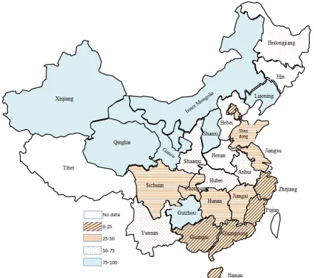
distribution of CO2 intensity in China is dramatically uneven. Generally speaking, from 1998 to 2010,

CO2 intensity increases sharply from the eastern coastal areas to the middle and western areas (Figure

1). In detail, six provinces with the lowest CO2 intensities were Guangdong (0.111 tons/billion yuan),

Hainan (0.115 tons/billion yuan), Fujian (0.116 tons/billion yuan), Beijing (0.134 tons/billion yuan),

Guangxi (0.153 tons/billion yuan), and Zhejiang (0.158 tons/billion yuan); whereas six provinces with

the highest CO2 intensities were Gansu (0.533 tons/billion yuan), Qinghai (0.536 tons/billion yuan),

Inner Mongolia (0.565 tons/billion yuan), Ningxia (0.664 tons/billion yuan), Guizhou (0.706

3 _{Roberts and Grimes (1997) is the only work we know that studies the connection of carbon intensity and economic}

tons/billion yuan), and Shanxi (1.034 tons/billion yuan).4 _{Hence, examining the provincial variations}

of CO2 intensity and identifying its driving forces are necessary to make and implement effective and

appropriate CO2 reduction policies.

Fig. 1 The distribution of provincial average CO2 intensities in China between 1998 and 2010

Note: The CO2 intensity data are compiled from the database of Energy Economic

Center at Renmin University of China (http://rucee.ruc.edu.cn)

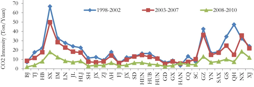
Observing Figure 2 that shows the changes in provincial CO2 intensities in China during the same

time period from 1998 to 2010, five patterns can be summarized. First, the CO2 intensity was unevenly

distributed across regions. It was relatively higher in the western and middle areas than in the eastern

areas, partly because most of the high energy-intensive industries were located in the western and

middle areas.

Second, the CO2 intensity evolved over time. It went down slightly during the period of 1995–

2002 compared to the period of 2003–2007 and dropped further in the period of 2008-2010. The

overall declining trend of CO2 intensity may imply that the CO2 emission reduction policies and

measures implemented in recent decades were effective and China may enter the low-carbon

industrialization process.

Third, CO2 intensity was diversified across provinces and the diversification was relatively greater

in the periods of 1995-2002 and 2003-2007 than in the period of 2008-2010. Taking the phase of

1998-2002 as an example, we can see that provinces like Sichuan, Hainan, Fujian, Guangdong,

Zhejiang, and Guangxi have relatively lower CO2 intensities, while provinces like Yunnan,

Heilongjiang, Jilin, Liaoning, Inner Mongolia, and Gansu have relatively higher CO2 intensities. Other

provinces, like Jiangsu, Shanghai, Beijing, Jiangxi, Hunan, Shandong, Henan, Hubei, Anhui, Tianjin,

Chongqing, Shanxi, Xinjiang, Ningxia, and Hebei, have middle-level CO2 intensities.

Fourth, CO2 intensity was spatially agglomerated. It can be seen that the differences in CO2

intensity across the eastern provinces were shrinking, indicating a pattern of agglomeration of low

energy-intensive industries there. There being far more highly energy-intensive industries

agglomerated in the middle/western regions than in the eastern region, thus the middle/western

regions have a much higher level of CO2 intensity than the eastern region.

Last, although the differences in CO2 intensities across the western provinces were still large in

general, the CO2 intensity in some western provinces, which are geographically close to the eastern

areas, has been approaching that of nearby eastern provinces, while this trend was not apparent in the

western provinces that are far away from the eastern provinces. This finding confirms our hypothesis

of spatial dependence.

Fig. 2 The provincial distribution of CO2 intensity between 1998 and 2010

Note: BJ = Beijing; TJ=Tianjin; HB =Hebei; SX = Shanxi; IM = Inner Mongolia; LN = Liaoning; JL = Jilin; HLJ = Heilongjiang; SH = Shanghai; JX = Jiangxi; ZJ = Zhejiang; AH = Anhui; FJ = Fujian; JX = Jiangxi; SD = Shandong; HEN = Henan; HUB = Hubei; HUN = Hunan; GD = Guangdong; GX = Guangxi; HAN =Hainan; CQ = Chongqing; SC = Sichuan; GZ = Guizhou; YN = Yunnan; SAX = Shaanxi; GS = Gansu; QH = Qinghai; NX = Ningxia; XJ = Xinjiang.

3 Model Specification

This study uses the dynamic spatial panel data model, which differs from the traditional panel data

model by taking into account both dynamic and spatial effects of provincial CO2 intensity. This model

has become popular in the last decade since it combines time series econometrics, spatial

0 10 20 30 40 50 60 70

BJ TJ _{HB SX IM LN} JL

HL

J

SH JX ZJ _AH FJ JX SD

HE

N

HUB HUN GD GX HA

N

CQ SC GZ YN _SAX GS QH NX XJ

CO2 In te n sit y (To n / Y ua n

econometrics, and panel econometrics. Elhorst (2012) points out that methods developed either for

dynamic but non-spatial or for spatial but non-dynamic panel data models all produced biased

estimates.

The dynamic spatial lag panel data model is traditionally specified as follows (Elhorst, 2010; Lee

and Yu, 2010; Zheng et al., 2013),

yit = α + θyi,t-1 + ρ∑j=1Wyjt + ∑kxit(k)βk + μi + υt + εit, i= 1,…, N; t = 1,…,T (3)

where yit is the dependent variable representing CO2 emissions intensity in province i at time t. W is a

non-stochastic, predetermined, contiguity-based binary matrix in which each element wij is set to be

one if provinces i and j (i ≠ j) share a common border, and zero otherwise. In addition, the matrix W

is commonly row-standardized such that the elements of each row sum to one. xit is a k × 1 vector of

independent variables. θ reflects the dynamic effects of CO2 intensity. ρ is the main concern of this

study and represents the spatial lag parameter that characterizes the strength of contemporaneous

spatial correlation between one province and other geographically proximate provinces. μi is the

provincial fixed effect, υt is the fixed temporal effect, and εit is the idiosyncratic disturbance term

assumed to be standard normal, independent of each other and everything else. When ρ = 0, Equation

(3) reduces to the traditional dynamic panel setting, while θ = 0 will reduce the model to the static

spatial econometric model.

In terms of econometric estimation, the most parsimonious panel model, or the static panel data

model which has neither dynamic effects nor spatial effects, can be estimated by the least-squares

dummy variables (LSDV) estimator if the spatial-specific effects can be considered as fixed effects, or

by the generalized lest-squares (GLS) estimator if the spatial-specific effects can be considered as

random effects (Hsiao 2003; Baltagi 2008). Extension of the static panel data model with a dependent

variable lagged in time (Yt-1) formulates a dynamic panel data model. The LSDV and GLS estimators

to estimate the dynamic panel data model become inconsistent if T is fixed, regardless of the size of

N (Arellano 2003; Baltagi 2008), which is because the lagged dependent term Yt-1 is correlated with

the spatial-specific effect.

The most popular approach to remove this inconsistency is generalized method of moments

(GMM). By creating a set of estimating equations for the parameters by making sample moments

match the population moments, one derives the estimators from the moment conditions, and also a

set exogenous variables (i.e., correlated with Yt-1 but uncorrelated with the errors) that can be used to

instrument Yt-1. The Anderson-Hsiao (1982) or Arellano and Bond (1991) difference GMM rests on

beyond (Y1, …, Yt-2, t ≥ 3) are used as instrumental variables for the differenced lagged dependent

variable (∆Yt-1). While the difference GMM approach can correct for the dynamic panel bias or

Nickell’s bias (1981) caused by the least squares regression that includes spatial-specific effects or the least squares dummy variable (LSDV) model, it may suffer from finite sample bias and precision

problems when the data series are persistent or are close to a random walk (Blundell and Bond, 1998),

as the instruments (i.e., Y1, …, Yt-2) are weak predictors of the endogenous changes (i.e., ∆Yt-1).

To overcome the drawbacks of the difference GMM approach, a closely related but improved

GMM dynamic panel approach, named system GMM, was proposed by Arellano and Bover (1995)

and later developed by Blundell and Bond (1998), which uses extra moment conditions that rely on

certain stationarity conditions of the initial observation. In other words, the system GMM approach

also uses lagged first differences for the equation in levels (i.e., the system GMM estimator also

instrument Yt-1 by the variables ∆Y1,…, ∆Yt-2, ∆X1,…, ∆Xt-1). Blundell and Bond (1998) argue that the

system GMM estimator performs better than the difference GMM estimator because of the following

properties: 1) increased efficiency; 2) less finite sample bias; 3) the instruments used in the level

equation model remain good predictors for the endogenous variables even when the series are very

persistent. Because of the good performance of the system GMM estimator compared with the

difference GMM estimator, it has become more popularly used in the panel data settings.

Ten years after the paper of Blundell and Bond (1998), several studies such as Kukenova and

Monteiro (2009) and Jacobs et al. (2009) extended the system GMM estimator of Blundell and Bond

(1998) to account for the spatial effects. The spatial system GMM is known to have the advantage on

avoiding the bias problem (especially with respect to the spatial autoregressive parameter, ρ) from the

spatial difference GMM estimator (Kukenova and Monteiro, 2009; Jacobs et al., 2009; Elhorst, 2010),

and over traditional spatial maximum likelihood estimation (MLE) in that the system GMM estimators

can also be used to instrument endogenous explanatory variables (other than Yt-1 and WYt). For this

reason, we will use the latter approach in this empirical study.

A few remarks are needed to better understand the spatial system-GMM estimator. First, the

number of sample observations is relatively large and the time span of interest is relatively short, as a

long time span would easily cause the over-identification problem of instrumental variables. The

sample in this study covers 30 provincial units from 1998 to 2010, so the first prerequisite could be

satisfied.5

5 _{It should be mentioned that dynamic panel is designed for micro-level panel data large N and small T. The available}

Second, the consistency of the system GMM estimator (and difference GMM estimator as well)

rests on the assumption that there is no first-order serial autocorrelation (i.e., AR(1) ≠ 0) in the error

terms of the level equation, or equivalently, there is no second-order serial autocorrelation (i.e., AR(2)

= 0) in the first-differenced errors. The Arellano and Bond (1991) test is used in this empirical work.

If the above assumption is violated, the instrumental variables can be highly correlated to the

endogenous variables and the model might not be specified correctly. One way to tackle this issue is

to add dependent variables of more than one lag in the model.

Third, the instrumental variables have to be relevant and valid, which implies that the following

two requirements have to be satisfied: 1) instrument relevance, under which the chosen instruments

have to be highly correlated with the endogenous regressors even after controlling for the exogenous

regressors. This requirement can be empirically tested in the first stage regression using a joint F test

of whether all excluded instruments are statistically significant, and 2) instrument exogeneity, which

can be tested using the Sargan (1958) or Hansen (1982) over-identification test in case there are more

excluded instruments than the number of endogenous variables.

Fourth, before implementing the spatial dynamic Blundell–Bond-type system-GMM regression,

it is necessary to test for the spatial interaction effects. In a cross-sectional setting, Anselin et al. (1996)

developed two Lagrange multiplier (LM) tests for spatially lagged dependent variables and for spatial

error correlation, and two robust counterparts of these two LM tests. For panel data setup, the first

two LM tests are: LM-LAG = [e′(IT W)Y/ 2]2/J, and LM-ERROR = [e′(IT W)e/ 2]2/(TTW),

where the symbol denotes the Kronecker product, I denotes the identity matrix, T is the order of

the matrix, and e denotes the estimated residual from the non-spatial dynamic panel model. J and TW

are defined as follows: J = [((IT W)X )′(INT−X(X′X)-1X′)(IT W)X + TTW 2]/ 2, and TW =

trace(WW + W′W). The two robust LM tests are defined as follows: Robust LM-LAG = [e′(IT

W)Y/ 2−e′_(I

T W)e/ 2]2/(J−TTW), and Robust LM-ERROR = [e′(IT W)e/ 2−TTW/J × e′(IT

W)Y/ 2_]2_/[TT

W(1 −TTW/J)]. Detailed derivations of these tests for a spatial panel data model with

spatial fixed effects can be found in Debarsy and Ertur (2010). Under the null hypothesis, these tests

follow a chi-squared distribution with one degree of freedom.

4 Data Source

 ˆ  ˆ



 ˆ  ˆ ˆ ˆ

 ˆ

  ˆ  ˆ 

ˆ

We used a panel data set of 30 provincial units (22 provinces, 4 municipalities, and 4 autonomous

regions) from 1998 to 2010.6 _{The dependent variable is the CO}

2 intensity, which is defined as the

provincial CO2 emissions divided by provincial GDP. Data on the provincial CO2 emissions during

the sample period are available from the Energy Economic Center at Renmin University of China

(http://rucee.ruc.edu.cn), where the CO2 emissions are calculated based on the method offered by

the Intergovernmental Panel on Climate Change (IPCC), and on other information, such as total

consumption of various energies, the heat content, the carbon content, and the carbon oxidation rate

of each energy, and so on.

The potential independent variables are identified as follows. GDP is an important factor that

affects CO2 intensity. Some empirical studies found that there exists a non-linear relationship between

GDP and the CO2 intensity. For instance, Roberts and Grimes (1997) found that the CO2 intensity

and per-capita GDP have an inverted U-shaped relationship, which indicates that CO2 intensity would

fall eventually as the economy develops even without any external reduction policies. Other studies

also found that the relationship can be N-shaped (Moomaw and Unruh, 1997; Friedl and Getzner;

2003; Millimet et al., 2003; Galeotti and Lanza, 2005; Yu et al., 2011). POP, indicating population size,

is another important factor that affects CO2 intensity. The larger the population size, the more direct

and indirect is energy consumption, and the greater the CO2 emissions. Historical data show that the

population and CO2 intensity are positively related. FDI measures foreign direct investment. The

relation between FDI and the CO2 intensity is ambiguous. On the one side, inward FDI takes into

account not only capitals but also advanced technologies, equipment, and management experience

invested in China. These investments help to improve the efficiency of energy consumption and

reduce pollution. Hence, FDI, to some extent, contributes to the decline of CO2 intensity in China.

On the other hand, the rise in exports due to FDI leads to the growth in implicit energy consumption

and hence CO2 emissions. Moreover, a large amount of FDI went into pollution-intensive industries,

which would result in an increase in CO2 intensity. Therefore, the relationship between FDI and CO2

intensity is not clear and deserves further empirical analysis.

SEC is measured as the ratio of value-added from the secondary industries to the total industry

value-added. Currently, the ratio of the primary, secondary, and tertiary industries in China is 1:5:4

(Yu et al., 2011) and the growth in the economy is heavily dependent on the secondary industries,

especially on the industries with high-energy consumption and high pollution. The CO2 emissions of

the secondary industries are much more than those of the primary and tertiary industries. Therefore,

we expect the coefficient of this variable to be negative. RD is defined as the ratio of research and

development (R&D) expenditure to GDP. R&D inputs can affect CO2 intensity in two respects. On

the one side, based on the endogenous growth theory, the advancement of technology (say,

low-carbon technology) improves the utilization of natural resources, so the resources could be saved and

recycled. From this point of view, science and technology innovation has a positive effect on the

reduction in CO2 intensity. On the other side, R&D expenditure might increase CO2 emissions

because the main concern of science and technology innovation is to increase output rather than to

reduce CO2 emissions. Therefore, the relationship between R&D and CO2 intensity is also

ambiguous.7

The data on the aforementioned variables, including GDP, POP, and SEC, are obtained from the

China Statistical Yearbook which is compiled by China Statistical Press. The FDI data come from the

CEIC Database.8 _{The R&D expenditure data are taken from China Statistical Yearbook on Science and}

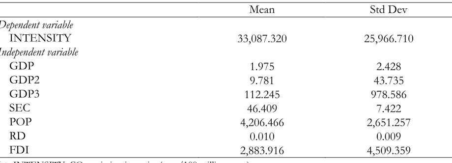
Technology. The variables used in the empirical model and their summary statistics are presented in

Table 1.

Table 1 Description and Statistics of Variables

Mean Std Dev

Dependent variable

INTENSITY 33,087.320 25,966.710

Independent variable

GDP 1.975 2.428

GDP2 9.781 43.735

GDP3 112.245 978.586

SEC 46.409 7.422

POP 4,206.466 2,651.257

RD 0.010 0.009

FDI 2,883.916 4,509.359

Note: INTENSITY: CO2 emission intensity (tons/100 million yuan)

GDP: per capita GDP (10 thousand yuan/person)

GDP2: GDP squared GDP3: GDP cubed

SEC: ratio of value-added from the secondary industry to total industry value-added (%) POP: population size (10 thousand persons)

7 _{It is worth mentioning though that R&}D’s scale is rather small compared with the product process, which implies that

even though R&D has positive or negative effect on carbon intensity, the effect may be true only in terms of statistical significance instead of economic significance.

8 _{CEIC is an euromoney institutional investor company (http://www.ceicdata.com/). CEIC Data provides the most}

RD: ratio of R&D expenditure to GDP (%) FDI: foreign direct investment (US $)

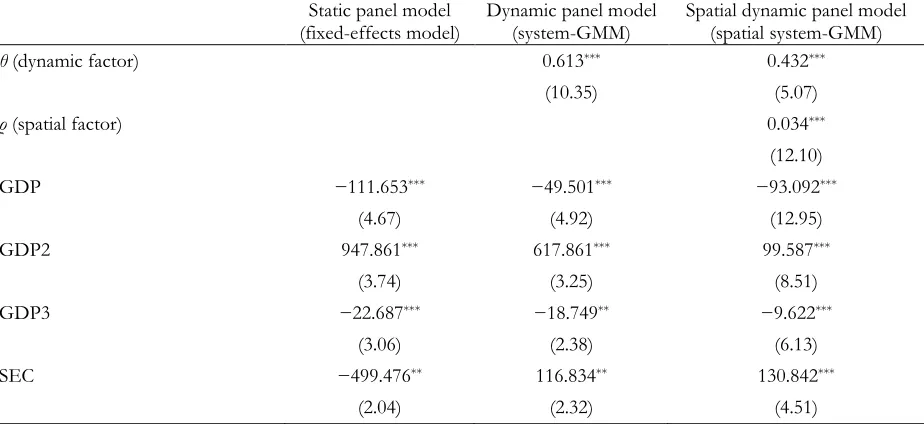
5 Empirical Findings

The base empirical results are shown in Table 2. Beginning with the static panel regressions in Table

2,9 _{the Hausman test statistics (21.38, p = 0.000) indicates that fixed effects model (FEM) is preferred}

to the random effects model. The coefficient regression results show that the coefficients of GDP,

GDP squared (GDP2), and GDP cubed (GDP3) are, respectively, negative, positive, and negative.

Besides, all estimates are statistically significant at the level of 1%. This result suggests that CO2

emission intensity and GDP are nonlinearly related, which is expected. Specifically, they have an

inverted N-shaped relationship rather than an inverted U-shaped relationship or a linear relationship.

Yet, population size and R&D are found to have neither positive nor negative effects on CO2 emission

intensity. Besides, a higher share of the secondary industry is negatively associated with CO2 emission

intensity. Certainly, this conflicts with theory. This is because the FEM model does not take into

account the endogeneity and dynamic attributes of the data.

Turning attention to the dynamic panel model (i.e., the system-GMM model) in Table 2, the

system GMM model accounts for endogeneity, but ignores spatial interactions across jurisdictional

CO2 emission intensities. The system GMM results are generally more plausible than those from FEM,

as evidenced by diagnostic tests for autocorrelation and Hansen test for over-identification.

Furthermore, the lagged parameter of CO2 emission intensity is positive and statistically significant,

suggesting evidence of dynamic nature of CO2 emission. GDP terms now have smaller (in absolute

value) relationship with CO2 emission intensity than was suggested by the FEM estimates. In addition,

share of the secondary industry is positively associated with emission intensity, R&D is negatively

related to emission intensity. These results are expected, while the negative and statistically significant

coefficient estimate for population size seems unexpected. Yet, like the FEM model, the system-GMM

model has problems of model specification. Particularly, the system-GMM estimates suffer from

omitted variable bias due to ignorance of spatial spillovers effect (or spatially lagged dependent

variable), as evidenced by Moran’s I and robust LM tests for spatial autocorrelation (Table 2).

9 _{We conducted the panel unit root tests (Levin, Lin and Chu (LLC, 2002), Im Pesaran and Shin (IPS, 2003), and Phillips}

and Perron (PP, 1988)) for the explanatory variables in this study. We found in general that GDP and FDI are I(1)

processes, while SEC and RD are I(0) processes. So eventually we assumed all variables are generated by a stationary

The last column of Table 2 shows the fully-specified spatial system-GMM results.10 _{The error}

term’s first-order serial correlation test, second-order serial correlation test, and Hansen over-identification test indicate that the system-GMM does not have the misspecification problem and that

the instrumental variables selected are indeed exogenous.11 _{The coefficient estimates for the CO} 2

emission intensity equation now reflect some major changes from non-spatial system-GMM and some

main results are summarized as follows.

First, the spatial lagged coefficient ρ is positive and statistically significant at the 1% level, which

indicates that the CO2intensities in the neighbouring provinces have a positive impact on one’s own

province’s CO2 intensity. Specifically, as the CO2 intensity in the neighbouring provinces rises on

(spatial) average by 1%, ceteris paribus, the CO2 intensity in the province of interest would rise by 0.03%.

Second, the inverted N-shaped relationship remains valid between CO2 intensity and GDP. Such

finding is not in line with the EKC literature, but is consistent with Moomaw and Unruh (1997), Du

et al. (2007), and Yu et al. (2011). Yet, a noteworthy change from the non-spatial model (FEM, or

system GMM) to the spatial system-GMM model is that GDP terms now have smaller (in absolute

value) relationships with CO2 emission intensity than was suggested by the FEM or system GMM

estimates.

Third, like the system-GMM estimate, a higher share of the secondary industry is positively

associated with CO2 emission intensity. This finding is predicted by theory as China’s economy is

heavily dependent on secondary industries, such as steel and iron, aluminium smelting, cement,

chemicals, and transportation industries, and these industries are also the ones that emit the most CO2.

Fourth, R&D remains to be statistically insignificant at the 10% level, implying that technological

innovation has no obvious effect on provincial CO2 intensities. This result is beyond our expectation.

The potential reasons can be three-fold: first, all levels of government are the leading forces of R&D

investment in China, some so-called ‘science and technology achievements’ fail to be converted into

production; second, the ratio of R&D expenditure to GDP may not be a good measurement of

technological innovations; and third, in the extensive economic growth stage, R&D expenditure in

China increased the CO2 emissions because the main concern of science and technology innovation

10 _{Analyses are done using STATA 12.0, a data analysis and statistical software, and some of the STATA modules to}

implement the diagnostic tests and spatial regressions are made by Emad Shehata (http://emadstat.110mb.com/ stata.htm).

11 _{Economic theory rarely gives us information about the lag length (Y}

t-1, Yt-2), which is usually determined empirically.

is to increase output rather than to reduce CO2 emissions. Hence, these factors combined make the

overall effect of R&D on provincial CO2 intensities insignificant.

Fourth, population size remains to be negative and statistically significant at 1% level. The

negative effect of population size, which seems puzzling at a first glance since it is usually believed

that more population leads to more energy consumption direct or indirectly and hence more CO2

emission (intensity), could imply that population size is associated with some agglomeration force that

could improve the production efficiency which leads to a reduction in emission intensity of carbon

dioxide. However, another noteworthy change is that the coefficient on population size from the

spatial system-GMM estimation decreases by almost three fold (from −3.54 to −1.28), suggesting that

system GMM without accounting for spatial dependence overestimates the population effect.

Last, most notably, FDI is now inversely related to CO2 intensity. As mentioned, the effect of

FDI on CO2 intensity is theoretically ambiguous, as, on the one side, FDI may reduce local CO2

intensity by introducing advanced technologies which help to improve the efficiency of energy

consumption; whereas, on the other side, FDI transfers some overseas high energy consumption

industries to China, which increases the overall consumption of energy and raises CO2 intensity. The

empirical findings show that the latter effect of FDI on CO2 intensity dominates the former. This

result is consistent with Yu (2012).

The striking changes from the FEM and system-GMM to the spatial system-GMM model point

to the adequacy of accounting for dynamic factor, endogeneity, spatial autocorrelation, and spatial

heterogeneity jointly.

Table 2 Determinants of Provincial CO2Emissions Intensity in China

Static panel model (fixed-effects model)

Dynamic panel model (system-GMM)

Spatial dynamic panel model (spatial system-GMM)

θ (dynamic factor) 0.613*** _0.432***

(10.35) (5.07)

ρ (spatial factor) 0.034***

(12.10)

GDP −111.653*** −_49.501*** −_93.092***

(4.67) (4.92) (12.95)

GDP2 947.861*** _617.861*** _99.587***

(3.74) (3.25) (8.51)

GDP3 −22.687*** −_18.749** −_9.622***

(3.06) (2.38) (6.13)

SEC −499.476** _116.834** _130.842***

POP −2.439 −3.543** −_1.283***

(0.97) (2.03) (6.71)

RD −141,487.115 172,590.853 −38,387.180

(0.33) (0.73) (0.62)

FDI 0.804* _{1.009 0.226}*

(1.85) (1.57) (1.78)

Constant 80,965.100*** _29,313.953*** _17,234.700***

(5.58) (3.05) (10.76)

Province dummy Y Y Y

R squares 0.341

Obs. 390 390 390

No. of provinces 30 30 30

Hausman test of fixed vs. random 21.38 [0.000] 8.97 [0.000]

Spatial Panel Autoregression Test

LM-Error Panel Test [0.111]

Robust LM-Error Panel Test [0.125]

LM-Lag Panel Test [0.023]

Robust LM-Lag Panel Test [0.057]

System GMM Test

AR(1) Test [0.007] [0.068]

AR(2) Test [0.403] [0.279]

Hansen Over-identification Test [0.998] [0.999]

Note: (i) ***, **, and * stand for the statistical significance at the level of 1%, 5%, and 10%, respectively; (ii) absolute t-values are in parentheses; (iii) p -values are in square brackets; (iii) spatial fixed or random effects are compared using Hausman’s specification test that is developed by Lee and Yu (2010).

6 Conclusions

Using a panel data set of 30 provincial units from 1998 to 2010, this study examined the determinants

and spatial nexus of the provincial CO2 intensities in China by estimating a spatial dynamic panel

(system-GMM) model. The dynamic factor, spatial dependence, and spatial heterogeneity of the

provincial CO2 intensities are rarely examined together in the existing literature. In this paper, we

found that provincial CO2 intensities are spatially dependent, CO2 intensity is increasing from the

eastern regions to the western regions, and the spatial agglomeration effects are obvious. In particular,

we found that CO2 intensities are spatially correlated across provinces, and the correlation tends to

increase over time. The Moran’s scatterplot shows that most provinces appeared in the first (HH) and

the third (LL) quadrants, which also reveals the spatial dependence, as it can be seen that provinces in

Yangtze River Delta region, provinces in the Pearl River Delta region, and Gansu, Ningxia, Inner

Mongolia, and Xinjiang provinces).

China’s CO2 intensity target that reducing the carbon emission by 40-45% in 2020 compared to

2005 is a big step in the right direction and it provides the right incentives for future improvements

in reducing emissions. Several policy suggestions on reducing CO2 intensity can be drawn based on

our empirical results. First, imposing a pollutant tax. Although energy or carbon tax is suggested by

numerous literatures, it can be a two-edged sword. On one hand, it contributes to reducing the demand

of coal and other energies that helps to cut down the CO2 emissions. On the other hand, it has negative

impact on energy-intensive industries as well as the macro-economy. Wei and Glomsrod (2002)

pointed out that if the government levy USD5 per ton of carbon as tax, the CO2 emission would be

reduced by 0.21 billion; meanwhile, the GDP would drop by 29 billion Chinese yuan in 2020. In other

words, the cost of reducing one ton of carbon emission is about 496 Chinese yuan (USD82.67) which

is much higher than USD5’s tax. Our finding of inverted N-shaped relationship between CO2

intensity and GDP shows that the environment can actually benefit from the growth of GDP. Thus,

it is preferable to levy tax based on pollutant directly, which is more efficient and relatively less harmful

to the economy. Also, we consider a progressive tax rate increment with a low initial tax rate will

mitigate the negative effects of tax on the economy. Furthermore, to compensate for the loss in GDP

resulted from pollutant tax, we suggest the central and local governments recycle the tax revenue by

cutting down energy-intensive industry’s production tax. In this case, pollutant tax brings a “double dividend” (improvement both in environment and economic efficiency).

Second, the spatial dependence found within in study implies that transboundary pollution

associated with CO2 emissions is potentially a real issue. This regional pollution problem is further

complicated by the fact that the coal consumed in some provinces is imported from other provinces.

The regional plans to reduce emissions then must inevitably involve energy trading. It is possible that

neighbouring provinces may develop cooperative initiatives to reduce emissions. Taking the CO2

emission quota as an example, central government should allocate the quota across provinces based

on the provincial factor endowments and allow for quota transactions among provinces. The

western/middle provinces have relatively larger CO2 emissions because most of the energy-intensive

industries are located there, so those provinces should have more of the quotas. Local governments

should make good use of their comparative advantages to improve energy utilization, which can not

Third, optimizing the industrial composition by enhancing the development of green industries

and constraining the development of high-carbon consumption industries. Meanwhile, positively

developing the environmental friendly alternative energy sources, such as solar energy, wind energy,

and hydro energy.

Fourth, enlarging the R&D investment aiming at recycling CO2 emissions besides improving

energy efficiency and reducing CO2 emission. We suggest governments of all levels earmark the

pollutant tax revenue as the R&D fund that is used exclusively for CO2 emission recycling and

reduction. We also recommend that governments should facilitate the cooperation between

energy-intensive industry and local universities as well as other research agencies to make a fully use of their

comparative advantage in research. Besides, governments should set up a supervision division to

guarantee the transfer of the research achievements into productivity.

Last but not least, fostering enterprises’ low-carbon production and creation consciousness.

Using proper policies to guide the enterprises to make correct choice between the low-carbon

technique and traditional business, as well as between the short-run profits and long-run development.

Moreover, encouraging the citizens to engage in energy-saving and emission-reduction activities and

constructing an intensive, economical, and ecological development trajectory. The bottom line is that

these policies, regulations or initiatives need to start being developed soon. Nonetheless, China’s

carbon intensity target still leaves room for even more ambitious action.

References

Anderson T, Hsiao C (1982) Formulation and estimation of dynamic models using panel data. J Econom 18: 47–82.

Anselin L (1991) Handbook of regional and urban economics: Peter Nijkamp, ed., Volume 1: Regional Economics

(North-Holland, Amsterdam, 1986). Reg Sci and Urban Econ 21(1): 143–156

Anselin L (1995) Local indicators of spatial association – LISA. Geogr Analy 27: 93–115

Anselin L, Bera A, Florax R, Yoon M (1996) Simple diagnostic tests for spatial dependence. Reg Sci and Urban Econ 26:

77–104

Arellano M (2003) Panel data econometrics. Oxford University Press.

Arellano M, Bond S (1991) Some tests of specification for panel data: Monte Carlo evidence and an application to

employment equations. Rev of Econ Stud 58: 277–297

Arellano M, Bover O (1995) Another look at the instrumental variable estimation of error-components models J of

Econom 68: 29–51

Baltagi B(2008) Econometric analysis of panel data. 4th edn., Chichester: John Wiley

Blundell R, Bond S (1998) Initial conditions and moment restrictions in dynamic panel data models. J Econom 87(1): 115–

143

Burnett J, Bergstrom J (2010) U.S. state-level carbon dioxide emissions: A spatial-temporal econometric approach of the environmental Kuznets curve. Faulty Series #96031 from Department of Agricultural and Applied Economics, University of Georgia

Cai F (2008) Lewis turning point: A coming new stage of China’s economic development. Social Sciences Academic Press

(China)

Chen S (2011) The carbon intensity’s downward fluctuation mode and economic explanations in China. World Econ 4:

Costantini V, Martini C (2006) A modified environmental Kuznets curve for sustainable development assessment using panel data. Working Papers 2006.148, Fondazione Eni Enrico Mattei

Dasgupta S, Laplante B, Wang H, Wheeler D (2002) Confronting the environmental Kuznets curve. J Econom Perspect

16(1): 147–168

Debarsy N, Ertur C (2010) Testing for spatial autocorrelation in a fixed effects panel data model. Reg Sci and Urban Econ

40: 453–470

Dinda S (2004) Environmental Kuznets curve hypothesis: A survey. Ecol Econ 49(4): 431–455

Du G, Cai Y, Li S (2010) The changing trend analysis of provincial carbon intensity from fossil energy in China between

1997 and 2007. Geogr and Geogr Inf Sci 5: 76–81 (in Chinese)

Du T, Mao F, Luo R (2007) An analysis of economic growth and CO2emission evolution. Chinese J Pop, Resour and Env

2: 94–99 (in Chinese)

Elhorst P (2010) Dynamic panels with endogenous interaction effects when T is small. Reg Sci and Urban Econ 40(5):

272–282

Elhorst P (2012) Dynamic spatial panels: models, methods, and inferences J Geogr Sys 14: 5–28

Fan D, Liu H (2012) The distribution characteristics and changes of provincial carbon intensity in China. J Xi'an Inst of

Finan and Econ 3: 4–10 (in Chinese)

Fan Y, Liu L, Wu G, Tsai H, Wei Y (2007) Changes in carbon intensity in China: Empirical findings from 1980 to 2003.

Ecol Econ 62(3-4): 683–691

Friedl B, Getzner M (2003) Determinants of CO2 emissions in a small open economy. Ecol Econ 45(1): 133–148

Galeotti M, Lanza A (2005) Desperately seeking environmental Kuznets. Environ Model and Soft 20(11): 1379–1388

Grossman G, Krueger A (1991) Environmental impacts of a North-American free trade agreement. NBER Working Paper 3914

Hansen L (1982) Large sample properties of generalized method of moments estimators. Econom 50: 1029–1054

Hsiao, C. (2003) Analysis of panel data. Cambridge University Press: Cambridge

Im S, Pesaran M, Shin Y (2003) Testing for unit roots in heterogeneous panels. J Econom 115: 53–74

Intergovernmental Panel on Climate Change (IPCC) (2007) IPCC fourth assessment report: climate change 2007. Cambridge University Press: Cambridge

Jacobs J, Ligthart J, Vrijburg H (2009) Dynamic panel data models featuring endogenous interaction and spatially correlated errors. International Center for Public Policy (formerly the International Studies Program) Working Paper Series 0915, Andrew Young School of Policy Studies, Georgia State University

Kahrl F, Roland-Holst D (2006) China’s carbon challenge: Insights from the electric power sector (available at

http://areweb.berkeley.edu/~dwrh/Docs/CCC_110106.pdf, accessed on March 14, 2013)

Kukenova M, Monteiro J (2009) Spatial dynamic panel model and system GMM: A Monte Carlo investigation IRENE Working Papers 09-01, Irene Institute of Economic Research

Lee L-F, Yu J (2010) Estimation of spatial autoregressive models with fixed effects, J of Econom 154: 165–185.

Levin A, Lin CF, Chu CSJ (2002) Unit roots tests in panel data: asymptotic and finite sample properties. J Econom 108:

1–24

Lin B, Jiang Z (2009) EKC forecasting and driving forces of China’s CO2. Manag Sci 4: 27–36

Lindsay H (2001) Global warming and the Kyoto Protocol. Environ Pol Iss (available at

http://www.csa.com/discoveryguides/ern/01jul/overview.php, accessed on March 14, 2013.

Liu L, Wang J, Wu G, Wei Y (2010) China’s regional carbon emissions change over 1997-2007. Inter J of Energy and Env

1: 161–176

Liu H, Zhao H (2012) The regional differences of CO2 intensity in China. Stat Res 6: 46–50 (in Chinese)

Millimet D, List J, Stengos T (2003) The environmental Kuznets curve: Real progress or misspecified models? Rev of

Econ and Stat 85(4): 1038–1047

Moomaw W, Unruh G (1997) Are environmental Kuznets curves misleading us? The case of CO2 emission. Environ Dev

Econ 4: 451–463

Moran, P (1950) Notes on continuous stochastic phenomena. Biometrika 37(1): 17–23

Narayan P, Narayan S (2010) Carbon dioxide emissions and economic growth: Panel data evidence from developing

countries. Energy Policy 38: 661–666

Nickell S (1981) Biases in dynamic models with fixed effects. Econometrica 49: 1417–1425

Panayotou T (1993) Empirical tests and policy analysis of environmental degradation at different stages of economic development World Employment Programme Research Working Paper WEP2-22/WP 238

Panayotou T (2000) Economic growth and the environment. CID Working Paper 56, Harvard

Phillips P, Perron P (1988) Testing for a unit root in time series regression. Biometrika 75, 335–346.

Roberts J, Grimes P (1997) Carbon intensity and economic development 1962-91: A brief exploration of the

SarganJ (1958)The estimation of economic relationship using instrumental variables. Econom 26: 393–415

Schmalensee R, Stoker T, Judson R (1998) World carbon dioxide emissions: 1950-2050. Rev Econ and Stat 80: 15–27

Soytas U, Sari R (2009) Energy consumption, economic growth, and carbon emissions: Challenges faced by an EU

candidate member. Ecol Econ 68: 1667–1875

Stern D (2004) The rise and fall of the environmental Kuznets curve. World Dev 32: 1419–1439

Tisdell C (2001) Globalisation and sustainability: Environmental Kuznets curve and the WTO. Ecol Eon 39: 185–196

Wang C, Chen J, Zou J (2005) Decomposition of energy-related CO2 emission in China: 1957-2000. Energy 30: 73–83

Wei T, Glomsrod S (2002) The impacts of carbon tax on Chinese economy and CO2 emission. World Econ and Polit 8:

47–49

Wu L, Kaneko S, Matsuoka S (2005) Driving forces behind the stagnancy of China’s energy-related CO2 emissions,

intensity change and scale change. Energy Policy 33: 319–335

____ (2006) Dynamics of energy-related CO2 emissions in China during 1980 to 2002: The relative importance of energy

supply-side and demand-side effects. Energy Policy 34: 3549–3572

Yu H (2012) The determinants and spatial nexus of provincial energy consumption intensity in China. Resour Sci 7: 1353–

1365 (in Chinese)

Yu Y, Zheng X, Zhang L (2011) Economic development, industrial composition, and CO2 intensity – A provincial panel

data analysis in China. Econ Theory and Bus Manage 3: 72–81(in Chinese)

Yue C, Hu X, He C, Zhu J, Wang S, Fang, J (2010) An analysis of provincial carbon emissions and carbon intensity in

China from 1995-2007 J of Peking Univ 46: 510–516 (in Chinese)

Zeng X, Pang H (2009) The CO2 emissions, trends, and emission reduction measures of Chinese provinces. China Soft

Sci (The Supplementary Issue) 8: 64–70 (in Chinese)

Zhao Y, Huang X, Zhong T (2011) The spatial evolution characteristics of CO2 intensity from energy consumption in

China from 1999 to 2007. Env Sci 11: 3145–3152 (in Chinese)

Zheng X, Zhang L, Yu Y, Lin S (2011) On the nexus of SO2 and CO2 emissions in China: the ancillary benefits of CO2

emission reductions. Reg Environ Change 11: 883–891

Zheng X, Li F, Song S, Yu Y (2013) Central government’s infrastructure investment across Chinese regions: A dynamic