Joint Closed Loop Power Control and Adaptive Beamforming for Wireless Networks with Antenna Arrays in a 2D Urban Environment

Wireless Sensor Network, 2010, 2, 869-878

doi:10.4236/wsn.2010.211105 Published Online November 2010 (http://www.SciRP.org/journal/wsn)

Joint Closed-Loop Power Control and Adaptive

Beamforming for Wireless Networks with Antenna Arrays

in a 2D Urban Environment

Mohamad Dosaranian Moghadam1_{, Hamidreza Bakhshi}2_{, Gholamreza Dadashzadeh}2 1

Department of Electrical Engineering, Islamic Azad University, Qazvin Branch, Qazvin, Iran

2

Department of Electrical Engineering, Shahed University, Tehran, Iran

E-mail: [email protected], [email protected], [email protected] Received July 25,2010; revised August 31,2010; accepted October 2,2010

Abstract

The interference reduction capability of antenna arrays and the power control algorithms have been consid-ered separately as means to decrease the interference in wireless communication networks. In this paper, we propose smart step closed-loop power control (SSPC) algorithm in wireless networks in a 2D urban envi-ronment with constrained least mean squared (CLMS) algorithm. This algorithm is capable of efficiently adapting according to the environment and able to permanently maintain the chosen frequency response in the look direction while minimizing the output power of the array. Also, we present switched-beam (SB) technique for enhancing signal to interference plus noise ratio (SINR) in wireless networks. Also, we study an analytical approach for the evaluation of the impact of power control error (PCE) on wireless networks in a 2D urban environment. The simulation results indicate that the convergence speed of the SSPC algorithm is faster than other algorithms. Also, we observe that significant saving in total transmit power (TTP) are pos-sible with our proposed algorithm. Finally, we discuss three parameters of the PCE, number of antenna ele-ments, and path-loss exponent and their effects on capacity of the system via some computer simulations.

Keywords: Adaptive Beamforming, Closed-Loop Power Control, Matched Filter, Urban Signal Propagation Simulator, Power Control Error

1. Introduction

Diversity and power control are two effective techniques for enhancing the signal to interference plus noise ratio (SINR) for wireless networks. Diversity exploits the random nature of radio propagation by finding inde-pendent (or, at least, highly uncorrelated) signal paths for communication. If one radio path undergoes a deep fade, another independent path may have a strong signal. By having more than one path to select from, the SINR at the receiver can be improved. The diversity scheme can be divided into three methods: 1) the space diversity; 2) the time diversity; 3) the frequency diversity. In these schemes, the same information is first received (or trans-mitted) at different locations (or time slots/frequency bands). After that, these signals are combined to increase the received SINR. The antenna array is an example of the space diversity, which uses a beamformer to increase the SINR for a particular direction [1]. Accordingly, the

their ability to separate the desired signal from interfer-ing signals. By knowinterfer-ing the direction of the desired sig-nals, they are able to adjust the antenna pattern intelli-gently by adjusting the weights of the adaptive algorithm [2-4].

On the other hand, power control can be realized by allocating different power levels to the links with differ-ent link gains. For example, links with smaller links gains are supposed to have larger power levels. This lar-ger power level may cause more interference to other users. Therefore, adequate power control is needed to meet the SINR requirement while minimizing the power consumption and increasing the capacity in all network. In general, two types of power control are often consid-ered. 1) Closed-loop power control 2) Open-loop power control [2,3]. In a closed-loop power control, according to the received signal power at a base station (BS), the base station sends a command to a mobile set to adjust the transmit power of the mobile. Also, closed-loop power control is employed to combat fast channel fluc-tuations due to fading. Closed-loop algorithms can effec-tively compensate fading variations when the power control updating time is smaller than the correlation time of the channel. However, in an open-loop power control, a mobile user adjusts its transmit power according to its received power in downlink [1-6].

The first goal of this paper is to extend our work in [7,8] by considering closed-loop power control and power control error (PCE). In [7], a constrained least mean squared (CLMS) algorithm was used for tracking mobile user in a 2D urban environment without power control algorithm. Also in [8], we proposed the SSPC algorithm in wireless network by the CLMS algorithm without considering the effect of PCE in 2D urban envi-ronment. Accordingly, in this paper we present smart step closed-loop power control (SSPC) algorithm for minimizing the total transmit power (TTP) in wireless networks [9]. On the other hand, the issue of the effect of power control errors on wireless networks has received a great deal of attention over the last few years [2,3]. Fi-nally, we consider the effect of PCE on wireless net-works in a 2D urban environment [10].

The organization of the remainder of this paper is as follows. In Section 2, propagation model in a 2D urban environment and also functional state of urban signal propagation simulator (USPS) are described. Section 3 considers the adaptive antenna array. The CLMS algo-rithm is summarized in Section 4. In Section 5, we pre-sent the SSPC algorithm. Then in Section 6, we extend the analysis to the case of PCE on wireless networks. Section 7 presents switched-beam (SB) technique and equal sectoring (ES) method. Finally, simulation results and conclusions are given in Sections 8 and 9.

2. Propagation Model

Because of using 2D urban structure in reverse link (up-link) in this work, for computing yield for path between a user and BS, propagation model in urban environments are dramatized. In propagation model in urban environ-ments and in reverse link, user antenna is radiating beams which are diffusing in all directions and parts of beams reach to BS.

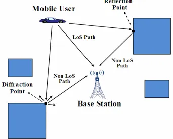
[image:2.595.339.510.545.682.2]

In urban environment, delivered beam from user by the time of collision to an obstacle like a wall surface or a building, reflects to a new angle and continues its path, this is called reflection phenomena. In condition when radiated beam is conflicted to a obstacle edge then dif-fraction phenomena is happened and diffracting point is diffusing new beams to all directions like a transmitter. All reflected beams, will stay in the environment till the time their power are not reduced to a threshold limit. Figure 1 shows both phenomena in reverse link. In this work, USPS dramatizing is used for implementing a 2D urban environment [7,11].

According to above dramatization, we could see be-cause of line of sight (LoS) in un-urban environment, only one signal is delivered from each user to receiver, while in function and because of elimination phenomena in an urban environment, beside to signals which are delivered to line sight, signals which have difference in phase or domain with this signal are also received by receiver.

3. Adaptive Antenna Array

An adaptive antenna array consists of a set of antennas, designed to receive signals radiating from some specific directions and attenuate signals radiating from other di-rections of no interest. The outputs of array elements are weighted and added by a beamformer, as shown in Fig-ure 2, to produce a directed main beam and adjustable

[image:3.595.108.487.78.246.2]

Figure 2. Antenna array and beamformer [13].

nulls. In order to reject the interference, the beamformer has to place its nulls in the directions of sources of inter-ference, and steer to the direction of the target signal by maintaining constant gain at this direction [12]. In this paper, we focus on the uplink communication path in a single-cell wireless system with M users and only one BS. Also we use a uniform linear array (ULA) of N an-tenna elements.

Accordingly, the received signal vector in BS can be written as [12]

 



    

1 M

i i i i

i

t p s t   t









 

x v n (1)

wheres ti

 

is the message signal transmitted from the

ith user; piis the received power of the ith user in BS

which is equal to p Gi i wherepiand Gi denote the

transmitted power of the ith user, and the link gain be-tween user i and BS in LoS path (or the best non-LoS path if LoS path is not exist), as shown in Figure 1, re-spectively. Also n

 

t is the thermal noise vector at the input of antenna array at BS and i is the

correspond-ing time delay. For simplicity, we further assume that the time delays for all uses are equal to 0. Also the N1 vectorvi

 

 is the array response for user i and can be

written as follows [12]:

 

,

 

, 1

i L

i i l i i l

l

  







v a (2)

where Li is the number of paths between user i and

BS in USPS; i l, is the direction of arrival (DoA) in the

lth path for user i; i l, is the normalized attenuation

by the best link gain (Gi) in USPS between user i and

BS in the lth path, therefore 0i l, 1. Also, response

of the base station array to the direction i l, is given by

 

, 1 exp



,



... exp



( 1) ,



T

i l i l

i i l  j j N  

a (3)

where j 1 and





, 2 / sin ,

i l d i l



     , in which  is signal wavelength and d is the distance between the antenna elements that for avoid the spatial aliasing should be defined as d0.5.

In non-spread spectrum systems, the transmitted signal is given by [12]

 

  



i i

m

s t 



b m g tmT (4)

where b mi

 

is the ith user information bit stream with

a bit period of T and g t

 

is the pulse-shaping filter impulse response. It has been shown that the output of a matched filter sampled at the symbol intervals is a suffi-cient statistic for the estimation of the transmitted signal. The matched filter is sampled at tmT

 

 

*

 

* t mT

m  t g t _

x x (5)

Hence, the received signal at the output of the matched filter is given by

 

   

   

 

   

 

 

1

M

i i i i k k k k

k k i

i i i i i

m p G b m p G b m

m p G b m m m

 



 

  

  



x v v

n v I n

(6) where Ii

 

m is the interference for user i in BS and

 

 

*

 

* t mT

m  t g t _

n n .

4. Constrained LMS Algorithm

combined form of the constraint is called constraint for narrowband beamforming [12-14].

This form consider a narrowband beamformer where the narrowband signal from each element of smart an-tenna are multiplied by the complex weight calculated by using narrowband adaptive beamforming algorithm, and then summed to produce the output of the array. The definition of the complex weights of this beamformer in the mth iteration for the ith user is as follows [13-15]:

 

(1)

 

(2)

 

( )

 

... N T

i m  wi m wi m wi m 

w (7)

Accordingly, the output of the array in the mth itera-tion for user i is given by

 

m

   

m m

y_i w_iH x

(8) The expected output power of the array in the mth it-eration is given by

 







   



       





 

 

2 _* E E E

i i i

H H H

i i i xx i

y m y m y m

m m m m m m



 w x x w w R w

(9) where E

 

. is denoted the expectation and Rxx is the

correlation matrix of the received signal vectorx

 

m . A real-time CLMS algorithm for determining the op-timal weight vector for user i is [13,14]:





 



 





, gmax



1

1

i i i

H

i i i

m m g m

        

w w w

w a (10)

where ai



i, g_max



denotes spatial response of the array

for user i in the best path gain, i.e., i l, 1, and



1



i m

w is the new weight computed at the



m1



th iteration for user i. Also, the variable scalar  de-notes a positive scalar (gradient step size) that controls the convergence characteristic of the algorithm, that is, how fast and how close the estimated weights approach the optimal weights, and g



wi

 

m



denotes an

unbi-ased estimate of the gradient of the power surface (wi

 

m HR wxx i

 

m which is the expected output power

of the array) with respect to wi

 

m after the mth

itera-tion. The algorithm is “constrained” because the weight vector satisfies the constraint at each iteration, that is



, max



1

H

i i i g 

w a . Rewrite the CLMS algorithm as fol-lows [14].







 



 



 

, max



1 i i g

i m i i m g i m

N  

   a

w β w w (11)

where



, max

 

, max



H

i i g i i g

i

N

 

 a a

β I (12)

The gradient of H

 

 

i m xx i m

w R w with respect to

 

i m

w is given by

 





*



 

 



2

 

H

i i xx i xx i

i

g m m m m

 _

   



w w R w R w

w

(13) and its computation using this expression requires knowledge of Rxx, which normally is not available in

practice. For a standard LMS algorithm, an estimate of the gradient at each iteration is made by replacing Rxx

by its noise sample xi



m1

 

xi m1



H available at time instant



m1



, leading to

 







  

*

2 1

i i i

g w m   x m y m (14) The CLMS is a fast convergence algorithm. However, it is drastically sensitive to the mismatch in the direction of arrival. Meanwhile, the weights estimated by the stan-dard algorithm are sensitive to the signal power, requir-ing a lower step size in the presence of a strong signal for the algorithm to converge, which in turn regarding the decrease of mis-adjustment error, the convergence time is increased [14-16].

Consider the problem of beamforming as to maximize the SINR for a specific link, which is equivalent to minimizing the interference at the receiver of that link. In order to minimize the variance or average power at the output of the beamformer subject to maintaining unity gain at the direction of the mobile user signal. Accord-ingly, we can rewrite the average output power for user

ias [12]

ˆH ˆ

i i xx i

 w R w (15) where ˆwi is the optimum weight vector for user i

with CLMS algorithm. If the message signals s ti

 

are

uncorrelated and zero mean, the correlation matrix Rxx

is given by

   

   

   

2 1 M H H

xx i i i i k k k k n

k k i H

i i i i i

p G p G

p G              



R v v v v I

v v Φ

(16) where

   

2 1

M

H

i k k k k n

k k i

p G   

 







Φ v v I (17)

is the correlation matrix of unwanted signals for user i in BS, and 2

n

 is the noise power at the input of each array element.

Combining (15)-(17), we obtain the received signal plus interference power as a function of weight vector

 

2

   

1

2

ˆ ˆ ˆ

ˆ ˆ

M

H H H

i i i i i k k i k k i

k k i H

n i i

p G p G

         



w v w v v w

w w

Accordingly, the SINR at BS for user i can be writ-ten as follows [12].

 





 

 

2

2 ₂

1

ˆ ˆ

SINR ,

ˆ ˆ ˆ

H

i i i i

i M

H H

k k i k n i i

k k i

p G

p G

 

 

 







w v w v

w v w w

(19)

In order to perform the bit error rate (BER), we as-sume Gaussian approximation for the probability density function of interference plus noise. The conditional BER for a BPSK modulation is [17]:

 



ˆ







ˆ

 





BER_i w v,  Q 2 SINR _i w v,  (20) where

 

1



2



exp / 2 2 x

Q x u du







_

 (21)

It should be mentioned that for the array antenna weight vector elements in the CLMS algorithm and for big, will converge after a few iteration (is approxi-mately equal to the number of beamformer weights, i.e.,mN) [7,16]. Moreover it is obvious that, without power control algorithm, the calculated optimal weight vector does not guarantee desirable SINR for the mobile user. Thus, we introduce our proposed algorithm in next section.

5. Smart Step Closed-Loop Power Control

Algorithm

A major limiting factor for the satisfactory performance of cellular systems is the near-far effect. Power control is an intelligent way of adjusting the transmitted powers in cellular systems so that the TTP is minimized, but at the same time, the user SINRs satisfies the system quality of service (QoS) requirements, [18,19].

Depending on the location where the decision on how to adjust the transmitted powers is made, the power con-trol algorithms can be divided into two groups: central-ized and distributed techniques [1-6,12]. In centralcentral-ized power control, a network center can simultaneously com-pute the optimal power levels for all users. However, it requires measurement of all the link gains and the com-munication overhead between a network center and base stations. Thus, it is difficult to realize in a large system [20]. Distributed power control, on the other hand, uses only local information to determine transmitter power levels. It is much more scalable than centralized power control. However, transmitter power levels may not be optimal, resulting in performance degradation [21,22].

The distributed closed-loop power control problem has been investigated by many researchers from many per-spectives during recent years [5,18,21-23]. For instance,

distributed conventional closed-loop power control strategy used in practice in wireless cellular systems as code divi-sion multiple access (CDMA) is a fixed-step controller based on SINR measurements. The fixed-step power con-trol (FSPC) algorithm is defined by [5]





1 *

sign

n n n

i i i i

p   p    (22) Where pin ,

* i

 andin are the transmitter power,

SINR target and measured SINR of user i at time n, respectively, and  is the fixed step size. Also pin 1



is transmitter power control (TPC) command in the feed-back link of BS to user i at time n1 (all signals are in decibels).

Also, the distributed traditional closed-loop power control (DTPC) is defined by [18]

* 1

n i n

i n i

i

p  p



 _

(23)

In both algorithms, the simple intuition behind this it-eration is that if the current SINR in of user i is less

than the target SINRi*, then the power of that user is

increased; otherwise, it is decreased.

It should be mentioned that convergence speed of DTPC algorithm is higher than FSPC algorithm. Also, the variance of the SINR mis-adjustment in FSPC algo-rithm is higher than DTPC algoalgo-rithm. But, it has been shown that the FSPC algorithm converges to

*

2

n

i i kd

    , where kd is the loop delay [4].

Also in [23], variable step closed-loop power control (VSPC) algorithm has been proposed. In this algorithm, variable step size is discrete with mode q. It is shown that the performance of VSPC algorithm with mode q = 4 is found to be worse than that of a fixed step algorithm (q = 1) under practical situations with loop delay of two power control intervals, but the convergence speed of VSPC algorithm is higher than FSPC algorithm. Also in this algorithm, the variance of the SINR mis-adjustment is reduced in compared to FSPC algorithm.

[image:6.595.122.477.517.683.2]

Figure 3. The slot at time nt is transmitted using power pn . The receiver measures SINR n over a number of pilots and/or symbols and derives a TPC command. The command is transmitted to the transmitter in the feedback link and the transmitter adjusts its power at time



n1



t according to the command. It should be mentioned that since the power control signaling is stan-dardized, the loop delays are known exactly [5].

In this paper, we propose smart step closed-loop power control algorithm for wireless networks. We ex-press the SSPC algorithm as follows [8,9].





1 * *

sign

n n n n

i i i i i i

p  p      (24) The algorithm is implemented as follows.

1) Select the initial transmitted power vector



n0



for all users as 0 0 0 0

1 2... M

p p p

 

  

p .

2) Estimate the weight vector for all users (wˆ_i,1 i M) with the CLMS algorithm using (11).

3) Calculate the SINR for all users (1 i M) at time n and after the time mN, according to the following equation:

 

 

2

2 ₂

1

ˆ

ˆ ˆ ˆ

n H

i i i i

n

i M

n H H

k k i k n i i

k k i

p G p G

 

 

 







w v

w v w w

(25)

4) If *

0

n

i i

   for each user then set n n 1 and calculate the TPC for all users at time n1 using (24) and go back to 2), where 0 is threshold value.

5) Finally, if *

0

n

i i

   for all users then algo-rithm ends.

As will be seen from simulation results, because of variable coefficient in the sign function, the convergence speed of our algorithm is higher than FSPC and VSPC algorithms.

6. Power Control Error

When imperfections in power control are considered, multipath fading is not perfectly compensated. As a re-sult, the power received from a mobile will not be con-stant at the base station to which the mobile is connected. Accordingly, we can be rewritten (1) as follows.

 



    

1 M

i i i i

i

t P s t   t







 

x v n (26)

where PE_b/T_b represents the received signal power of all users in the presence of PCE and Eb is the energy

per bit for all users. The variable i is PCE for user i,

which is assumed to follow a log-normal distribution and thus it can be written as 10i/10

i 

  , where i is a

Gaussian random variable with mean 0 and variance 2 

 for all users [3]. On the other hand, E

 

i for all users

can be written as follows [24].

 

2 2_{/ 2}

E _i e  ₍₂₇₎

where ln 10 / 10

 

. Accordingly, we can be rewritten the SINR in (19) as follows [10].

 





 

 

2 2

2

2

2

/ 2 2

1

ˆ

SINR , ,

ˆ

ˆ ˆ ˆ

i i

H

i i

M

H H

i k n i i

k k i

Pe Pe 





 

 



 

 







w v

w v

w v w w

(28)

7. Switched-Beam Technique and Equal

Sectoring Method

One simple alternative to the fully adaptive antenna is the switched-beam architecture in which the best beam is chosen from a number of fixed steered beams. Swit- ched-beam systems are technologically the simplest

and can be implemented by using a number of fixed, independent, or directional antennas [25]. We list the conditions of the SB technique for this paper as follows [11].

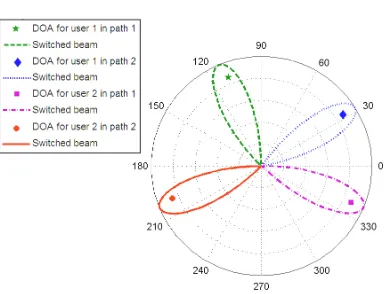
1) According to Figure 4, beams coverage angle is 30and overlap between consecutive beams is20. Thus each base station has 36 beams.

2) According to Figure 5, each user can be use one beam for its each path to communicate with a base sta-tion at any time.

One simple method to sectorize a cell is equal sector-ing; in which all sectors have the same coverage angle. In this paper, we assume three sectors for each base sta-tion with sector angle 120 for the ES method [26].

8. Simulation Results

[image:7.595.314.536.381.506.2]

In this section, we evaluate the performance of our algo- rithm by simulating the same system as in [7] with CLMS algorithm, SB technique, and ES method. For this purpose, we use part of two-dimensional map of the University of Toronto campus area in Canada as shown in Figure 6 [7]. According to this figure, we observe beside desired user, M 1 interference users in a stable positioning situation with uniform distribution are also

Figure 4. 36 beams in BS with the SB technique.

Figure 5. Select of beam for two users in two different paths with the SB technique.

sending information to BS equipped to an array antenna in reverse link. According to the description in Section 2, sending information by all users to BS is performed by dramatizer USPS. Also note that the variance of the noise (n2) for every element is assumed to be equal to

0.01; resolution and path loss in USPS R = 1 and 0.05dB/m

L , respectively; gradient step size in the CLMS algorithm 0.005; fixed step size for SSPC, FSPC, and VSPC algorithms  0.05; mode q4 for VSPC algorithm [23]; threshold value in SSPC algo-rithm 00.1dB; number of elements antenna array

10

[image:7.595.101.243.391.527.2]

N ; initial value for transmitted power vector for all usersp0 0; and the SINR target value is the same for all users and is set to *8 9 dB





. It also is assumed that the distribution of users is uniform.

[image:7.595.76.268.547.694.2]

Figure 7 shows the comparison of the average SINR achieved over M 15 users versus the power control iteration index (n) for SSPC, VSPC (q4), and FSPC algorithms and CLMS, SB, and ES techniques. Also in this simulation, we assume that each user to have a maximum power constraint of 1watt. It should be men-tioned that in case of without power control (PC), the transmitted power for all users is 1 watt [7]. Accordingly, we observe that the convergence speed of the SSPC al-

Figure 6. Two-dimensional map of the University of To-ronto campus area and placing users and base station con-tain array antenna in map center [7].

[image:7.595.316.534.561.695.2]

gorithm is faster than the VSPC and FSPC algorithms. For example, the SSPC algorithm (for CLMS algorithm) converges in about eight iterations, while VSPC and FSPC algorithms converge in about 11 and 16 iterations, respectively. Also this figure shows that the SSPC algo-rithm with SB technique converges faster than CLMS and ES methods. Also we observe that the SINR level achieved is below the target SINR value for ES method, because in this case the interference is higher than the other methods.

Figure 8 shows the comparison of TTP usage versus the power control iteration index (n), as Figure 7. But in this simulation, we assume that users no have maxi-mum power constraints. Similar to Figure 7, we observe that the ES method never can achieve the target SINR value for all users. Also this figure shows that the SSPC algorithm offers more savings in the TTP as compared the FSPC and VSPC algorithms. Also the TTP for the joint SSPC algorithm and SB technique is lower than other cases. Although not shown in the figure, in case of without power control and because of near-far problem, the target SINR level is not achieved for all users.

Figure 9 presents the average BER versus the signal to noise ratio (SNR) for CLMS algorithm and SB tech-nique and different values of _2. In this figure, we ob-serve that the average BER for the SB technique is lower than the CLMS algorithm. For example, at a SNR of 10 dB and _2 4 dB, the average BER is 0.0011 for CLMS algorithm, while for SB technique is 0.00018. Also it can be seen that the average BER for _2 0 dB (perfect power control) is lower than the other cases. For example, at a SNR of 10 dB and for CLMS algo- rithm, the average BER is 0.0007 for PPC, while for

2

8 dB



  the average BER is 0.0016.

Figure 10 presents the average BER versus the num-ber of active users for SNR10 dB and different val-ues of _2 as Figure 9. Similar to Figure 9, we observe that the average BER for _2 0 dB is lower than

2

2, 4,8 dB



  . For example, at a BER of 0.001, the

re-Figure 8. Total transmit power of all users versus power control iteration index (n). No power constraints.

Figure 9. Average BER versus the SNR for the SB tech-nique and CLMS algorithm (M = 15).

Figure 10. Average BER versus the number of active users for the SB technique and CLMS algorithm (SNR = 10 dB).

ceiver with CLMS algorithm support M 18users for

2 _{0 dB}



  , while for 2 _{2, 4,8 dB} 

  supportM 16, 15, and 12 users, respectively. Accordingly in this case, with

2 

 from 2 to 8 dB, the system capacity degrades from 6% to 34% compared to the case of PPC. We also ob-serve that with SB technique can achieve lower BER than the CLMS algorithm. For example, at a BER of 0.0001 and 2 _8dB



  , the number of users allowed in the system is M 15 users for SB technique, while for CLMS algorithm is M 5 users.

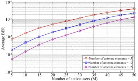
Other results displayed in Figure 11 and Figure 12 show the influence of path-loss parameter in USPS

 

L and number of antenna elements

 

N on the average BER for the CLMS algorithm, SNR10 dB, and 2



 4 dB

[image:9.595.62.284.80.206.2]

Figure 11. Influence of path-loss parameter (L) on average

BER (SNR = 10 dB, N = 10).

Figure 12. Influence of number of antenna elements (N) on

average BER (SNR = 10 dB, L = 0.05 dB/m).

9. Conclusions

In this paper, we studied performance of single-cell wireless communication systems in a 2D urban environ-ment with closed-loop power control. Also, we deter-mined the optimum weights of the elements of array an- tenna with the CLMS algorithm.

Accordingly, we proposed the SSPC algorithm in or-der to compensate the effects of the near-far problem. It has been shown that, by using antenna arrays at BS, this algorithm will decrease the interference in cell. In addi-tion, the TTP expected by all users is less as compared to the VSPC and FSPC algorithms. Thus, it decreases the BER by allowing the SINR targets for the users to be higher, or by increasing the number of users supportable at a fixed SINR target level. It has also been observed that the TTP in SB technique is less than CLMS algo-rithm. Also, it has been shown that the convergence speed of the proposed algorithm is increased in com-parison with the VSPC and FSPC algorithms. Also, our simulations show that the variations in power level due to PCE have a detrimental effect on system performance.

10. Acknowledgements

This research is supported under research project by the

Islamic Azad University, Qazvin Branch, Qazvin, Iran.

11. References

[1] J. T. Wang, “Admission Control with Distributed Joint Diversity and Power Control for Wireless Networks,”

IEEE Transactions on Vehicular Technology, Vol. 58, No.

1, 2009, pp. 409-419.

[2] A. Abrardo and D. Sennati, “On the Analytical Evalua-tion of Closed-Loop Power-Control Error Statistics in DS-CDMA Cellular Systems,” IEEE Transactions on

Vehicular Technology, Vol. 49, No. 6, 2000, pp. 2071

-2080.

[3] L. Carrasco and G. Femenias, “Reverse Link Perform-ance of a DS-CDMA System with both Fast and Slow Power Controlled Users,” IEEE Transactions on Wireless

Communications, Vol. 7, No. 4, 2008, pp. 1255-1263.

[4] L. Qian and Z. Gajic, “Variance Minimization Stochastic Power Control in CDMA System,” IEEE Transactions on

Wireless Communications, Vol. 5, No. 1, 2006, pp. 193-

202.

[5] M. Rintamaki, H. Koivo and I. Hartimo, “Adaptive Closed-Loop Power Control Algorithms for CDMA Cel-lular Communication Systems,” IEEE Transactions on

Vehicular Technology, Vol. 53, No. 6, 2004, pp. 1756

-1768.

[6] J. Wang and A. Yu, “Open-Loop Power Control Error in Cellular CDMA Overlay Systems,” IEEE Journal on Se-lected Areas in Communications, Vol. 19, No. 7, 2001, pp. 1246-1254.

[7] M. Dosaranian-Moghadam, H. Bakhshi, G. Dadashzadeh and P. Rahmati, “Adaptive Beamforming Method Based on Constrained LMS Algorithm for Tracking Mobile Us-er,” IEEE Global Mobile Congress, Shanghai, China, October 2009, pp. 1-6.

[8] M. Dosaranian-Moghadam, H. Bakhshi and G. Dadash-zadeh, “Adaptive Beamforming Method Based on Closed -Loop Power Control for DS-CDMA Receiver in Multi-path Fading Channel,” Accepted for publication in the

IEEE International Conference on Communication Sys-tems, Singapore, 17-20 November 2010.

[9] M. Dosaranian-Moghadam, H. Bakhshi and G. Dadash-zadeh, “Interference Management for DS-CDMA Systems through Closed-Loop Power Control, Base Station As-signment, and Beamforming,” Journal of Wireless Sensor Network, Vol. 2, No. 6, 2010, pp. 472-482.

[10] M. Dosaranian-Moghadam, H. Bakhshi, G. Dadashzadeh and M. Godarzvand-Chegini, “Joint Base Station Assign-ment, Power Control Error, and Adaptive Beamforming for DS-CDMA Cellular Systems in Multipath Fading Channels,” Accepted for publication in IEEE Global

Mo-bile Congress, Shanghai, China, 18-19 October 2010.

[image:9.595.59.286.248.381.2]

[12] F. Rashid-Farrokhi, L. Tassiulas and K. J. Ray-Liu, “Joint Optimal Power Control and Beamforming in Wireless Networks using Antenna Arrays,” IEEE Transactions on

Communications, Vol. 46, No. 10, 1998, pp. 1313-1324.

[13] M. Z. Shakir and T. S. Durrani, “Narrowband Beam-forming Algorithm for Smart Antennas,” International Bhurban Conference on Applied Sciences & Technology, Islamabad, January 2007, pp. 49-54.

[14] X. Y. Sun, X. H. Lian and J. J. Zhou, “Robust Adaptive Beamforming Based on Maximum Likelihood Estima-tion,” International Conference on Microwave and

Mil-limeter Wave Technology, Nanjing, China, Vol. 3, 2008,

pp. 1137-1140.

[15] J. Litva and T. Kwok-Yeung, “Digital Beamforming in Wireless Communications,” Artech House, London, 1996. [16] S. Haykin, “Adaptive Filter Theory,” 3th Edition,

Pren-tice Hall, New Jersey, 1996.

[17] R. L. Peterson, R. E. Ziemer and D. E. Borth, “Spread-Spectrum Communications,” Prentice-Hall, New Jersey, 1995.

[18] A. Yener, R. D. Yates and S. Ulukus, “Interference Management for CDMA Systems through Power Control, Multiuser Detection, and Beamforming,” IEEE

Transac-tions on CommunicaTransac-tions, Vol. 49, No. 9, 2001, pp. 1227

-1239.

[19] S. Kandukuri and S. Boyd, “Optimal Power Control in Interference-Limited Fading Wireless Channels with Outage Probability Specifications,” IEEE Transactions on Wire-less Communications, Vol. 1, No. 1, 2002, pp. 46-55.

[20] S. Grandhi, R. Vijayan and D. Goodman, “Centralized Power Control in Cellular Radio Systems,” IEEE

Trans-actions on Vehicular Technology, Vol. 42, No. 4, 1993,

pp. 466-468.

[21] J. Zander, “Distributed Cochannel Interference Control in Cellular Radio Systems,” IEEE Transactions on Vehicu-lar Technology, Vol. 44, No. 3, 1992, pp. 305-311.

[22] S. Grandhi, R. Vijayan and D.Goodman, “Distributed Power Control in Cellular Radio Systems,” IEEE

Trans-actions on Communications, Vol. 42, No. 2/3/4, 1994, pp.

226-228.

[23] A. Kurniawan, “Effect of Feedback Delay on Fixed Step and Variable Step Power Control Algorithm in CDMA Systems,” IEEE International Conference on Communi-cation Systems, Singapore, Vol. 2, 2002, pp. 1096-1100. [24] J. M. Romero-Jerez, C. Tellez-Labao and A. Diaz-Estrella,

“Effect of Power Control Imperfections on the Reverse Link of Cellular CDMA Networks under Multipath Fad-ing,” IEEE Transactions on Vehicular Technology, Vol. 53, No.1, 2004, pp. 61-71.

[25] B. Allen and M. Beach, “On the Analysis of Switch-ed-Beam Antennas for the W-CDMA Downlink,” IEEE

Transactions on Vehicular Technology, Vol. 53, No. 3,

2004, pp. 569-578.