Variance Estimation for High Dimensional Varying Index Coefficient Models

ISSN Online: 2161-7198 ISSN Print: 2161-718X

DOI: 10.4236/ojs.2019.95037 Oct. 8, 2019 555 Open Journal of Statistics

Variance Estimation for High-Dimensional

Varying Index Coefficient Models

Miao Wang

*

_{, Hao Lv, Yicun Wang}

Department of Statistics, School of Economics, Jinan University, Guangzhou, China

Abstract

This paper studies the re-adjusted cross-validation method and a semiparamet-ric regression model called the varying index coefficient model. We use the profile spline modal estimator method to estimate the coefficients of the pa-rameter part of the Varying Index Coefficient Model (VICM), while the un-known function part uses the B-spline to expand. Moreover, we combine the above two estimation methods under the assumption of high-dimensional data. The results of data simulation and empirical analysis show that for the varying index coefficient model, the re-adjusted cross-validation method is better in terms of accuracy and stability than traditional methods based on ordinary least squares.

Keywords

High-Dimensional Data, Refitted Cross-Validation, Varying Index Coefficient Models, Variance Estimation

1. Introduction

The variance estimate, in this paper, is the residual variance of the model. In the process of statistical modeling, the variance estimation of the model has been extensively studied. Most of the research methods are simple two-stage method, in the first stage, the important variables in the model are selected by the method of variable selection; in the second stage, the variance is estimated by the ordi-nary least squares method. In the first phase, the traditional variable selection method has two criteria, namely the Akaike Information Criterion (AIC) and the Bayesian Information Criterion (BIC). These two traditional methods use the empirical likelihood method to select the model with the smallest AIC and BIC values. At the same time, the variables contained in the model are the se-lected optimal variables. However, this variable selection method is neither

con-How to cite this paper: Wang, M., Lv, H. and Wang, Y.C. (2019) Variance Estima-tion for High-Dimensional Varying Index Coefficient Models. Open Journal of Statis-tics, 9, 555-570.

https://doi.org/10.4236/ojs.2019.95037

Received: September 11, 2019 Accepted: October 5, 2019 Published: October 8, 2019 Copyright © 2019 by author(s) and Scientific Research Publishing Inc. This work is licensed under the Creative Commons Attribution International License (CC BY 4.0).

http://creativecommons.org/licenses/by/4.0/

DOI: 10.4236/ojs.2019.95037 556 Open Journal of Statistics tinuous nor ordered. Therefore, the variance of the model estimated by the tra-ditional method will be large. Moreover, with the development of technology, high-dimensional data is applied to all aspects of life. The number of variables increases exponentially, and the calculation of the above two criteria also shows an exponential increasing trend, so the above method cannot be applied to high- dimensional data.

In the past research, many important variable selection methods such as LASSO (Least Absolute Shrinkage Selection Operator) and SCAD (Smoothly Clipped Absolute Deviation) have been proposed. LASSO was proposed by Tib-shirani (1996) [1]. For more details, see Fan and Peng (2004), Zhao and Yu (2006), Bunea (2007), Zhang and Huang (2008), Lv and Fan (2009), Fan and Lv (2011), and Kim (2008) [2]-[8]. In this method, a penalty term is added on the basis of the ordinary least squares method, and the coefficient value is reduced to 0, so that the corresponding variable is excluded from the model. Another type of variable selection tool is DS (Dantzig Selector). This method was first pro-posed by Candes and Tao (2005) [9] and can be easily reshaped into a linear model. Fan and Lv (2008) [10] sort the covariance matrix between covariate and response variables, and then select the first few variables with the largest correla-tion coefficient to complete the variable seleccorrela-tion. This method is called SIS (Sure Independence Screening). In later studies, some scholars extended the SIS, namely the iterative SIS (ISIS) method: the regression analysis was performed using the variables and dependent variables selected by SIS, and the regression residuals were replaced with response variables. Then continue to use the SIS method for a new round of variable selection. And repeat the above steps until all the important variables. For details, see Fan et al. (2009) [11]. After screening out the important variables, the second step of the simple two-stage method is generally calculated by least squares method. However, in order to overcome the root cause of the dimension, many scholars study the variance estimation in the case of high-dimensional data. Fan et al. proposed a re-adjusted cross-validation method (RCV) in 2012 to improve the simple two-stage approach. It is proved that the variance estimated by this method is stable and accurate. Zhao et al. (2014) [12] studied the variance estimation of linear models under certain as-sumptions. Reid, Tibshirani, Friedman (2016) [13] studied the model residual estimation in LASSO regression and performed a large number of simulations. They considered that the variance estimation of the residual sum of squares based on adaptive regularization parameter selection has the properties of finite samples.

DOI: 10.4236/ojs.2019.95037 557 Open Journal of Statistics model is more suitable. The literature research on semi-parametric models is mostly focused on the introduction of new models, such as linear models, add-on models, and so on. Hastie and Tibishirani (1993) [14] proposed the Variable Coefficient Model (VCM), which has been widely used in practical ap-plications. In addition, some scholars studied the single index coefficient model (SICM). The Variable Coefficient Single Index Model (VICSIM) was proposed by Wong et al. (2008) [15]. Ma and Song (2014) [16] proposed the varying index coefficient model for the first time, which has overcome the problems that the variable coefficient model cannot solve. Most scholars apply variable selection methods such as SIS, LASSO, and SCAD to the parametric model, while the method used in nonparametric estimation are kernel estimation, local linear kernel estimation, and spline functions. For the estimation of semi-parametric regression models, such as partial linear regression model, variable coefficient model, single-index model, etc., the parameter part is estimated by Profile Least Square Estimation (PLSE), and its non-parametric part is still using the previous non-parametric method. For example, Xue and Liang (2010) [17] used the PLSE method of kernel estimation when estimating the non-parametric part of the single-index model. However, there are few literatures on varying index coeffi-cients proposed in 2015, and the related estimation algorithms mainly use the profile least squares estimation method with B-spline to estimate the variable coefficient index model. Lv et al. (2016) [18] improved the PLSE, proposed a robust estimation procedure combining the logarithmic regression and the B-spline, and established the large sample property of the parameter estimation. The estimation of the unknown coefficient β is estimated by the profile spline modal estimator method (PSME). Moreover, in order to obtain the progressive distribution of the unknown function m Zl

( )

, they also proposed a two-stage

method of local linear kernel estimation.

The rest of the paper is organized as follows. In Section 2, we briefly introduce the varying index coefficient model, including the estimation method, the statis-tical inference of the coefficients, and the RCV estimation of the model. In Sec-tion 3, simulaSec-tion studies are conducted to evaluate the finite sample perform-ance of the proposed methods. In Section 4, a real data set is analyzed to com-pare the proposed methods with the existing methods. A discussion is given in Section 5.

2. Methodology

2.1. Varying Index Coefficient Models

DOI: 10.4236/ojs.2019.95037 558 Open Journal of Statistics

( )

1

d

l l

l

Y m Z X ε

=

=

∑

+ _(2.1) where Y is a response variable, X =

(

X1, , Xp

)

T and Z∈

[ ]

0,1 (for simplic-ity) are explanatory covariates, m

( )

⋅ =

(

m1

( )

⋅ , , mp

( )

⋅

)

T is a p-dimensional vector of the unknown coefficient functions, and model error

ε

_{is independent} of

(

X Z,

)

with mean zero and finite variance _σ2_{. The variable coefficient} model of Equation (2.1) faces two challenges in the case of today’s complex data. First, the variable Z has little effect relative to Y, so the interaction between the variables Z and X is difficult to detect; second, in many complex situations, Z is multi-dimensional, for example, studying the effects between chemical con-stituents. Thus, the coefficient function m Zl

( )

in the VCM model will fall into the dimension curse. To overcome these two problems, Ma and Song proposed the Varying index Coefficient Model (VICM) in 2015. The varying index coeffi-cient model is as follows:

(

)

(

T

)

1

, , d l l

l

Y m Z X β ε m Z β X ε

=

= + =

∑

+ _(2.2)

where βl=

(

βl1, , βlp

)

T is the coefficient of the variable Z and βlk is the co-efficient of Zk in Z. The introduction of the varying index coeffcient model was based on Ma and Song’s study of this biomedical project that affects chil-dren’s growth rates.

2.2. Estimation Procedure for the VICM

The estimation of the varying index coefficient models has two main aspects: one is the estimation of the parameter part β _{, and the other is the estimation of}

the function coefficient m ul

( )

l of the non-parametric part. In this paper, the

estimation of the unknown coefficient β _{is estimated by the profile spline}

modal estimator method (PSME). Once β _{is fixed, the unknown function}

co-efficient m ul

( )

l is estimated using B-spline. The specific estimation process of

the varying index coefficient models is as follows.

Let

{

(

X Z Yi, , ,1i i

)

≤ ≤i n

}

be the independent and identically distributed samples from model (2.2). Our main interest is to estimate the coefficient vec-tors βl and the non-parametric functions ml

( )

⋅ for l=1, , d. The

estima-tion of βl and ml

( )

⋅ in VICM is equivalent to maximizing

(

)

1

T

1 1

1 d d

h i l i l il

i Y l m Z X

n = φ = β

 ₋ 

 

 

∑

∑

(2.3)

subject to the constraint βl =1 and β >l1 0, where 1

( )

( )

1

1 1

h t h t h

φ

₌ −

φ

_,

t

φ

is a kernel density function symmetric about 0 and h1 is a bandwidth which determines the degree of robustness of the estimate. We use the standard normal density for φt throughout this paper to simplify the calculation. We use a basic approximation to estimate nonparametric functions. That is, we approximate

( )

l

DOI: 10.4236/ojs.2019.95037 559 Open Journal of Statistics B-spline basis functions of order q q

(

≥2

)

, where Jn=Nn+q and Nn is the number of interior knots for a knot sequence

1 0 q q1 Nn q 1 Nn q1 Nn 2q

ξ == =ξ <ξ ₊ <<ξ ₊ < =ξ _{+ +} ==ξ ₊ ,

where Nn increases along with the sample size n. Consider the distance be-tween two neighboring knotsHi = −ξ ξi i−1 and H =max1≤ ≤i Nn+1

{ }

Hi . Then, there exists constants C0 such that

_{{ }}

0

1 1

min _{i Nn i}

H _C

H

≤ ≤ +

< ,

{

}

( )

1

1 1

max≤ ≤i N_n Hi+ −Hi =o Nn− . Let Ul

( )

β

l =ZT

β

l, without loss of generality, we assume that Ul

( )

βl is confined in a compact set

[ ]

0,1 . Then,

nonparamet-ric functions m ul

( )

l can be approximated by

( )

( ) ( )

T

l l q l l

m u ≈B u

λ β

_, l=1, ,_ d _(2.4) where λ βl

( )

=

(

λ βs l,

( )

:1≤ ≤s Jn

)

T. Let

( )

(

( )

( )

)

T

T T

1 , , d

λ β

=

λ β



λ β

. Based on the above approximation, the objective function (2.3) becomes

( )

(

)

2 , ,

1 1 1

1 n d Jn

h i s q il l s l il

i l s

Y B U X

n = φ = = β λ

 

−

 

 

∑

∑∑

. (2.5)

Subsequently, we estimate the parameter vectors βl and the nonparametric functions ml

( )

⋅ in two steps below.

Step 1. Given β_{, we obtain estimate}

λ β

ˆ

( )

_of λ β

( )

by maximizing the objective function (2.5). Then, the estimator of m ul

( )

l can be obtained by

(

)

( ) ( )

( ) ( )

T

, ,

1

ˆ ˆ

ˆl l, Jn s q l s l q l l

s

m u β B u λ β B u λ β

=

=

∑

= _{. (2.6)}

In order to obtain efficient estimators of β, the “remove-one-component” method is employed. Specifically, for βl =

(

βl1, , βlp

)

T, let

(

)

T , 1 2, ,

l l lp

β - = β  β

be a p−1 dimensional vector by removing the 1st component βl1 in βl for all 1≤ ≤l d _{. Then} β_{l can be rewritten as}

( )

2 _T T

, 1 1 , 1 , , 1

l l l l l

β =β β ₋ =_ − β ₋ β ₋ _

  ,

2

, 1 1

l

β

− < . (2.7)

Thus, βl is infinitely differentiable with respect to

β

l, 1− and the Jacobian

matrix is

2

, 1 , 1

, 1 ₁

1

T

l l l

l

l _p

J

I

β β β

β ₋ − −

−   ∂ _− − _ = =   ∂  

, (2.8)

where Ip is the p p× identity matrix. We denote

(

)

T

T T

1 l, 1, , d, 1

β

− =

β

− 

β

−

and reformulate the parameter space of β−1 as follows:

(

)

{

_T T 2 ₁

}

1

β

1

β

l, 1:1 l d :

β

l, 1 1,

β

l, 1 Rp−

− − − − −

Θ = = ≤ ≤ < ∈ _{. (2.9)}

Let β β β=

( )

−1 with

β

l=

β β

l

( )

l, 1− for 1≤ ≤l d . Since the estimation

procedure of β requires estimates of both ml and its first order derivative l

DOI: 10.4236/ojs.2019.95037 560 Open Journal of Statistics is given by

(

)

,

( ) ( )

, , 1

( )

,

( )

1 2

ˆ

ˆ _, Jn Jn _ˆ

l l s q l s l s q l s l

s s

m u β B u λ β B − u ω β

= =

=

∑

 =

∑

 (2.10)

where ωˆs l,

( ) (

β = q−1

)

{

λ βˆs l,

( )

−λˆs l−1,

( )

β

}

(

ξs q+ −1−ξs

)

for 2≤ ≤s Jn. Thus, one has

(

)

( )

T

( )

, 1 1ˆ

ˆ_{s l l, q l l}

m u

β

=B− u D

λ β

, where Bq−1

( )

ul =

(

Bs q, 1−

( )

ul : 2≤ ≤s Jn

)

T and

(

)

( )

1 2 1 2

2 3 2 3

1

2 1 2 1 ₁

1 1 _{0 0}

1 1 0 0 1 1 1 0 0 n n q q q q

N q N q N q N q _{J J}

D q

ξ ξ ξ ξ

ξ ξ ξ ξ

ξ ξ ξ ξ

+ + + + + − + + − + _{− ×} −    _{− −}     ₋   _{− −}  = _{−  }     −    _{− −}            .

Step 2. After this re-parametrization, combine with the estimators ml and ˆ_l

m for l=1, ,_ d_{, we can construct the profile spline modal objective function} for the parametric components. Then, we can obtain the estimator βˆ−1 of β−1 by maximizing Ln

(

β β

( )

−1

)

over β−1∈ Θ−1, where

( )

(

1

)

2 ,

(

( )

)

,

( )

1 1 1

1 n d Jn

n h i s q il l s l il

i l s

L Y B U X

n

β β₋ φ β λ β

= = =

 

=  − 

 

∑

∑∑

, (2.11)

which is equivalent to solve the following estimating equations:

( )

(

)

( )

(

)

( )

( )

(

)

(

( )

)

( )

{

}

( )

(

)

(

( )

)

( )

{

}

1 1

2 , ,

1 1 1

T T

1 1 1 1 1 1, 1

T T , 1 1 _ˆ ˆ ˆ _, ˆ ˆ _, 0 n n J n d

h i s q il l s l il

i l s

i i i i

d id d id d i d i

L

Y B U X

n

m U X J Z D

m U X J Z D

β β β

φ β λ β

β β λ β β β

β β λ β β β

− − = = = − − ∂ ∂   = −  −     _{+ ∂ ∂}      ×     + ∂ ∂     =

∑



∑∑

   (2.12)

where Di

( )

β =

(

Di sl,

( )

βl ,1≤ ≤s Jn,1≤ ≤l d

)

T with

( )

(

( )

)

, ,

i sl l s q il l il

D

β

=B U

β

X _, mˆ ,_l

( )

⋅

β

is given in (2.10) and φh2 is the first

derivative of φh2. We obtain the estimate of β−1, say, βˆ−1 and then obtain βˆ

via the transformation (2.7). Thus, we call the estimator βˆ as the profile spline modal estimator (PSME).

3. Simulation Studies

3.1. Results in Finite Sample

per-DOI: 10.4236/ojs.2019.95037 561 Open Journal of Statistics formance of the proposed methodology. We generate data from the following VICM:

(

)

(

T

)

(

T

)

(

T

)

1 1 1 2 2 2 3 3 3

, ,

i i i i i i i i i i i

Y m Z X=

β

+ =

ε

m Z

β

X +m Z

β

X +m Z

β

X +

ε

_(3.1) with Xi =

(

X X Xi1, i2, i3

)

T, where Xi is generated from Bernoulli (p = 0.5), and

(

X Xi2, i3

)

T is drawn from a bivariate normal distribution with mean 0, variance 1, and covariance 0.2. To generate Zi=

(

Z Z Zi1, i2, i3

)

T, we first sample

(

_{* * *}

)

T 1, 2, 3 i i i

Z Z Z from a multivariate normal with mean 0, variance 1, and covari-ance 0.2, and then let

( )

* _{0.5, 1,2,3}

ik ik

Z = Φ Z − k= _{, where} Φ ⋅

_{( )}

is the CDF of the standard normal. The true loading parameters are set as

(

)

T

1 1 2,1,3₁₄

β = ,

(

)

T 1 1 3,2,1₁₄

β = _{, 1} 1 2,3,1

(

)

T 14

β = _{. Set}

( )

*

( )

{

*

( )

}

l l l l l l

m u =m u −E m u _, l=1, 2,3

where *

( )

( )

{

( )

}

1 1 10exp 5 1 1 exp 5 1

m u = u + u , *

( )

( )

2 2 5sin π 2

m u = u , and

( )

{

( )

(

)

}

*

3 3 3 sin π 3 cos 2π 3 4π 3

m u = u + u − _{. Finally,} Y_i, 1≤ ≤i n_{, are generated} from the VICM (3-1), where

(

T T T

)

T

1, ,2 3

β

=

β β β

, and errors εi follow

(

)

(

_0, 2 _,

)

i i

N

σ

Z X _with 2

(

_,

)

{

₁₀₀

(

_{, ,}

)

}

{

₁₀₀

(

_{, ,}

)

}

i i i i i i

Z X m Z X m Z X

σ

= −

β

+

β

_.

Although the estimation process of the varying index coefficient model is in-troduced in Section 2.2, it is still difficult to directly estimate (2.12). Therefore, an iterative calculation algorithm is needed to estimate the unknown parameters and the unknown function coefficients. The specific algorithm is divided into the following two steps:

Step 1. The initial value

(

β β β1, ,2 3

)

of β is obtained in the following four steps:

1) Assuming that the unknown function ml is a linear function, then

(

)

(

T

)

1

, , d

i i l l i l il

i

m Z X β a b Z β X

=

=

∑

+ _.

2) The estimated value

(

a vˆ ˆl, l

)

of

(

a vl, l

)

is estimated by minimizing

(

T

)

2

1 1

n d

i l l i il

i l

Y a v Z X

= =

 _{− +} 

 

 

∑

∑

, and thus the expression 0

(

)

( )

1 2

ˆ_{l v vˆ ˆl l sgn vˆl}

β

= _is

obtained, where vˆ1l is a part of vˆl. 3) Let ˆ Tˆ0

l i l

U =Z β , then obtain the initial unknown function ˆini

( )

l

m ⋅ _from

the varying coefficient model

( )

1

ˆ d

l l l

l

Y m U X ε

=

=

∑

+ _.

4) Obtain β1ini by minimizing

(

)

2

1 T

1 1

ˆ

2 n n ini

i l i l il i Y l m Z X

β − = =  ₋     

∑

∑

, i.e. the initial value.

DOI: 10.4236/ojs.2019.95037 562 Open Journal of Statistics

[16]. Under certain assumptions, the estimated parameters satisfy the following asymptotic properties:

(

)

(

)

(

)

(

)

(

)

( )

1 2

0 1 0

1 1

1

1 2 0

1

ˆ _{, ,}

, , , 1

n

i i i

n

i i i i i p

i

n n X Z

n Y m Z X X Z o

β β β

β

− ⊗ −

− −

= −

=

 

− = Φ 

 

 

×_ − Φ _+

 

∑

∑

(3.2)

where

(

_{, ,} 0

)

{

(

( )

0 _, 0

)

T

}

T_,1

i i l l l l l l

X Z β  m U β β X J Z l d

Φ =_ ≤ ≤ _

   , and

( )

Z Z P Z= − _{in the above expression. Here} Z can be estimated by

( )

n

Z Z P Z= − _{, where}

( )

0

(

( )

)

1

1

ˆ ˆ

ˆ ,

d

n k J l l

l

P Z g U β β X

=

=

∑

_{. (3.3)}

The estimation procedure of 0

( )

1 ˆ

ˆJ ,

g ⋅β _{in Equation (3.3) is similar to the}

es-timation of the unknown function mˆ ,l

( )

⋅βˆ , except that the response variable Y is replaced by Zk in the iterative estimation process. According to the asymp-totic properties (3.2) we can get an equation and use this equation for iterative calculations. The iteration stops when the absolute difference (dif) from the last calculated unknown parameter is less than 10-4 _{or the iteration number (iter) is} greater than or equal to 100.

According to the idea of the above specific algorithm, we use R (64-bit) to write four functions such as Design matrix, transform, Jac, vicmest. Among them, vicmest is the main program for estimating unknown parameters, and the other three functions are intermediate conversion functions. First, we calculate the initial value β β β1, ,2 3 of β through the first step. The results are shown

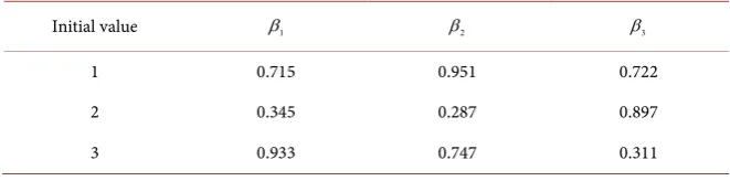
in Table 1. It can be seen from Table 1 that the initial value calculated by Step 1

is consistent with the trend of the actual value, but the deviation from the actual value is still large. Therefore, it is necessary to further calculate the estimated value by the second step. At this point, by running the four programs such as vicmest, the result of stopping the main program after 64 iterations is finally ob-tained, and _{dif =8.45267 10×} −6 _{at this time. The specific calculation results of}

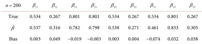
[image:8.595.208.539.644.726.2]

the estimated values βˆ of β and their deviations are shown in Table 2. It can be seen from Table 2 that the value of a estimated by the profile spline mo-dal estimator (PSME) is better, the deviation from the actual value (Bias) is smaller, and the mean deviation is less than 5%.

Table 1. The initial values of β _{calculated by step 1.}

Initial value β1 β2 β3

1 0.715 0.951 0.722

2 0.345 0.287 0.897

[image:9.595.208.538.92.164.2]

DOI: 10.4236/ojs.2019.95037 563 Open Journal of Statistics

Table 2. The estimated value of β and its deviation from the true value.

200

n= β11 β12 β13 β21 β22 β23 β31 β32 β33

True 0.534 0.267 0.801 0.801 0.534 0.267 0.534 0.801 0.267

ˆ

β 0.537 0.316 0.782 0.798 0.538 0.271 0.461 0.833 0.305 Bias 0.003 0.049 −0.019 −0.003 0.003 0.004 −0.074 0.032 0.038

From the main program vicmest, not only can the estimated value βˆ be ob-tained, but also can we obtain gamm0, which is the coefficient after the expan-sion of the B-spline basis function. Bring the calculated βˆ and the coefficient gamm0 into the Formula (2.10), get the value of the unknown function mˆ ,l

( )

⋅β and the predicted value of the response variable Y. The results of the gamm0 co-efficient are shown in Table 3. An estimate of mˆ ,l

( )

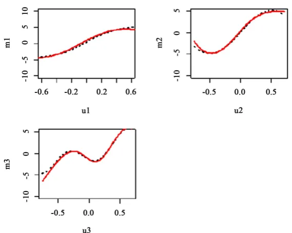
⋅β can be seen from Figure

1, where the red curve represents the estimate and the black curve represents the actual value. It can be seen intuitively from Figure 1 that the fitting effect of the B-spline expansion is very good, not only the general trend of the unknown non-parametric function is well maintained, but also the accuracy of the estima-tion is relatively high. As shown in Table 4, we calculate the root mean square error of the coefficient of mˆ ,l

( )

⋅β by further calculation. It can be seen from

Table 4 that the unknown function has a small deviation, and the RMSE is less

than 0.28, which indicates that the estimation effect is better. Moreover, Y can be calculated after obtaining the estimated values βˆ and mˆ ,l

( )

⋅β . Finally, the variance of error of the model (3.1) is calculated to be 5.777.

3.2. Results in High-Dimensional Case

In this section, we numerically simulate the variance estimation of the varying index coefficient model in high-dimensional conditions.

The profile spline modal estimator (PSME) shows good estimation variance under low-dimensional data settings. However, in the case of high-dimensional data, it will fall into the dimension curse, and the deviation of the estimated variance will increase as the dimension increases. The re-adjustment cross-validation method proposed by Fan et al. (2012) [19] can be considered as an effective way to overcome the dimension curse in high-dimensional problems through theo-retical proof and data simulation test. Naturally, this paper applies the re-adjusted cross-validation method (RCV) to the high-dimensional varying index coeffi-cient model for the first time. There are two types of covariates in the varying index coefficient model (2.2). The first type is Z. If Z is from a single variable, its relationship with the covariate X is more difficult to detect. The second type of variable is the covariate X. What we are concerned about is the estimation of the variance of the varying index coefficient model when the first type of covariate Z is high-dimensional.

[image:10.595.231.516.67.294.2]

DOI: 10.4236/ojs.2019.95037 564 Open Journal of Statistics

[image:10.595.208.540.349.428.2]

Figure 1. Plots of the estimated nonparametric curves.

Table 3. The coefficient of the B-spline basis function.

1

i

B Bi2 Bi3 Bi4 Bi5 Bi6

1i

B −4.444 −4.808 −3.0887 3.912 5.004 3.973

2i

B −2.083 −6.179 −4.543 4.683 5.185 4.876

3i

B −6.294 −2.710 3.652 −5.970 7.624 5.766

Table 4. Root mean square error (RMSE) of mˆ ,l

( )

⋅β .

( ) 1

ˆ ,

m ⋅β mˆ ,₂( )⋅β mˆ ,₃( )⋅β

RMSE 0.349 0.222 0.258

type of covariate Z is set to a high dimensional variable. Where

( )

* _0.5

ik ik

Z = Φ Z − _, k=1,2, ,_ d_{, that is, Z is a d-dimensional covariate. The} setting of m ul

( )

l and the error term is also the same as model (3.1).

[image:10.595.208.537.465.500.2]

DOI: 10.4236/ojs.2019.95037 565 Open Journal of Statistics The idea of SIS makes high-dimensional model selection possible, greatly speeding up the selection of variables, and making model selection problems ef-ficient and modular. The SIS variable selection method can be used in conjunc-tion with any model selecconjunc-tion technique. Fan et al. (2010) [20] apply the SIS method to the Cox proportional hazard model. The Cox proportional hazard model is similar to the varying index coefficient model mentioned in this paper. They are all nonlinear models and both have the need to estimate the coefficients of the nonparametric function and its parameter parts. Therefore, we believe that in the case of high-dimensional data, it is feasible to use the SIS method to make the first variable selection of the varying index coefficient model.

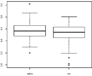
We use the SIS method proposed by Fan et al. (2008) [10] to select variables. The number of variables selected is tentatively 20. The calculation process is simulated using R software. We have written VicmRCV and the vicmest func-tion for the estimafunc-tion of the RCV process. The data simulafunc-tion process was re-peated 100 times, and a box plot of the variance as shown in Figure 2 was ob-tained. In the figure, naïve represents a simple two-stage approach, while rcv represents a re-adjusted cross-validation method.

[image:11.595.221.529.442.695.2]

It can be seen from Figure 2 that in the d dimension (the dimension of the variable Z, is as high as 100), the sample size is only 200, the variance of the re-adjusted cross-validation (RCV) two-stage method is better than the simple two-stage method. However, the calculated error variance value is large. To some extent, the estimation method of the estimated varying index coefficient model mentioned in Section 3.1 of this paper is not accurate enough and not robust enough as the estimated error variance value is large.

Figure 2. Box plot of the variance calculated by using the simple two-stage method and

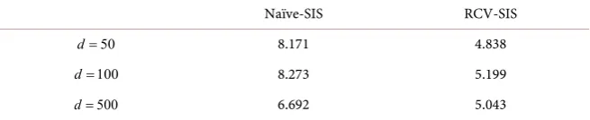
DOI: 10.4236/ojs.2019.95037 566 Open Journal of Statistics As shown in Table 5, changing the values of p and n gives more simulation results. Table 5 compares the normal two-stage method (Naive-SIS) with the RCV two-stage method (RCV-SIS) at n=100_, d=50,100,500_{. By comparing} the root mean square error estimated by the two estimation methods, we find that the mean square error (MSE) of the RCV two-stage estimation is smaller in each dimension than the MSE estimated by the ordinary two-stage method. That is, the model estimated by the RCV method is more accurate. But from Table 5, we can also find other laws. Conventionally, as the dimension p increases, the estimated accuracy decreases, which results in the root mean square error be-comes larger. However, from the results of Table 5, this law is completely inap-plicable in the ordinary two-stage method. When the dimension comes to maximum (d =500_{), the root mean square error is the smallest, and its value is}

6.692. When d=100_{, the MSE is the largest with a value of 8.273. In}

conclu-sion, the order is disorganized, and the mean square error does not become lar-ger as the dimension becomes larlar-ger in general cases.

In fact, it is not difficult to explain this phenomenon because in the variable selection phase, for the SIS method, we select the variables with the co-correlation coefficients ranked in the top twenty (descending order). Since the fixed value 20 is small relative to the covariate, the probability of selecting all important vari-ables is relatively low. From the data in the RCV-SIS column in Table 5, it can be seen that the SIS method is much more stable after combining RCV. At d = 50, the estimated MSE is the smallest with value of 4.838. In the case of three different dimensions, the error estimated by the RCV method is smaller than the mean square error estimated by the ordinary two-stage method.

4. Real Data Analysis

In this section, we will use the data collected by the Mayo Clinic. These data were obtained from trials conducted by the Mayo Clinic in primary biliary cir-rhosis (PBC) from 1974 to 1984. Specific data can be found in the R language Survival package. The dataset included 424 PBC patients who were referred to the Mayo Clinic during the decade between 1974 and 1984. The data met the randomized placebo-based eligibility criteria.

[image:12.595.211.539.656.723.2]

In the data set, the first 312 patients participated in the randomized trial while the other 112 patients did not participate in the clinical trial, but agreed to re-cord the basic measurements and follow the medical recommendations. Six of the above samples lost follow-up shortly after diagnosis. Thus there are 106 cases and 312 random participants. We preprocessed the data set via R software.

Table 5. Mean Square Error (MSE) for two different estimation methods at n=100.

Naïve-SIS RCV-SIS

50

d= 8.171 4.838

100

d= 8.273 5.199

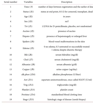
500

DOI: 10.4236/ojs.2019.95037 567 Open Journal of Statistics We first remove some samples with missing values. The number of samples that were eventually brought into the calculation after deletion was 276. The specific variables are described in Table 6.

As can be seen from Table 6, the response variable Y is the survival time of the patient. Since the difference among the response variables Y is large, we logarithmically convert the time Y to reduce the error. There are three covariates of X, which are the patient’s state X1 (Status), the patient’s age X2 (Age), and the patient’s gender X3 (Sex). Here we need to explain why we want to add gender variables. The gender variable was added because Huang Siyu (1985) [21] found that the incidence of men with primary biliary cirrhosis (PBC) was much lower than that of women. Therefore, we can know that gender has a great relationship with PBC. Another type of covariate Z has a total of 15 variables including al-bumin (alal-bumin), alkaline phosphatase (alk.phos), triglyceride (Trig), and plate-let count (Plateplate-let). Therefore, the varying index coefficient model constructed in this section is as follows:

( )

i

(

, ,

)

I 3 l 15 ld* ld il i

l d

Ln Y =m Z X β +ε = m _ Z β _X +ε

 

[image:13.595.203.528.368.734.2]

∑

∑

. (4.1)

Table 6. Interpretation of experimental variables in primary biliary cirrhosis (PBC).

Serial number Variables Description

1 Time (Y) number of days between registration and the earlier of death 2 Status (X1) status at end point, 0/1/2 for censored, transplant, dead

3 Age (X2) in years

4 Sex (X3) m/f

5 Trt (Z1) 1/2/NA for D-penicillmain, placebo, not randomised 6 Ascites (Z2) presence of ascites

7 Hepato (Z3) presence of hepatomegaly or enlarged liver 8 Spiders (Z4) blood vessel malformations in the skin 9 Edema (Z5) 0 no edema, 0.5 untreated or successfully treated _{1 edema despite diuretic therapy} 10 Bili (Z6) serum bilirubin (mg/dl)

11 Chol (Z7) serum cholesterol (mg/dl) 12 Albumin (Z8) serum albumin (g/dl) 13 Copper (Z9) urine copper (ug/day) 14 alk.phos (Z10) alkaline phosphotase (U/liter)

15 Ast (Z11) aspartate aminotransferase, once called SGOT (U/ml) 16 Trig (Z12) triglycerides (mg/dl)

DOI: 10.4236/ojs.2019.95037 568 Open Journal of Statistics Since the covariate Z has different physical meanings and different dimen-sions, it is meaningless to simulate the model at this time. So we need to elimi-nate the effects of different dimensions of the data through transformation. Therefore, these 15 variables should be standardized before the specific calcula-tion, which is Z-Score standardization.

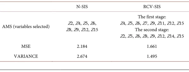
Through previous studies, we have roughly learned that variables such as se-rum bilirubin content (Z6), albumin content (Z8), urinary copper content (Z9), alkaline phosphatase content (Z10), prothrombin time (Z14) have a strong rela-tionship with the response variable Y. We first use the SIS method to select the variables with the first 8 covariate correlations, and then use the simple two-stage method and the re-adjusted cross-validation (RCV) two-stage method to estimate the coefficient β of the covariate Z and the model variance. The results are shown in Table 7.

As can be seen from Table 7, when using SIS for variable selection, the im-portant variables such as Z6 and Z9 are selected three times. Important variables have strong correlations in theoretical analysis. From this aspect, it can be seen that the SIS variable selection method can select all important variables with a high probability to a certain extent. The RCV can repeatedly select variables by selecting the first missing variable or deleting the extra variable that was selected for the first time. The model variance estimated by the RCV-SIS two-stage method is significantly better than the N-SIS simple two-stage method. In the high-dimensional case, the re-adjusted cross-validation method (RCV) has a better performance in the varying index coefficient model. The root mean square error and the resulting variance are smaller than the simple two-stage es-timate. Therefore, the RCV-SIS two-stage method is more accurate in predicting the survival time of patients, and can provide more reasonable guidance and ad-vice for follow-up medical treatments.

5. Discussion

In this paper, we study a new class of semiparametric regression models: varying index coefficient models. The estimation of the unknown coefficient β _is

[image:14.595.211.533.618.741.2]

es-timated by the profile spline modal estimator method (PSME), while the un-known non-parametric function part is expanded with the B-spline. After studying the gradual nature of the coefficients, we estimate the coefficient β

Table 7. PBC dataset estimation results.

N-SIS RCV-SIS

AMS (variables selected) _{Z8, Z9, Z12, Z15} Z2, Z4, Z5, Z6,

The first stage: Z4, Z5, Z6, Z7, Z9, Z11, Z12, Z15

The second stage: Z2, Z5, Z6, Z8, Z9, Z12, Z14, Z15

MSE 2.184 1.661

DOI: 10.4236/ojs.2019.95037 569 Open Journal of Statistics using an iterative method. With data simulation, we found that the estimated

β of this method has a small deviation, and the unknown function part of the B-spline estimation has a good fitting effect as well. Finally, under the setting conditions of high-dimensional data, we carried out a two-stage RCV estimation of the varying index coefficient model. We find that the variance and mean square error estimated by the RCV method are superior to the simple two-stage method. In the final empirical phase, it was originally intended to model the PBC data using a survival model (semi-parametric varying coefficient additive risk model). However, through research literature, it is known that gender vari-ables and state varivari-ables are closely related to the survival time of patients with primary biliary cirrhosis. The variable Z has a certain relationship with the three variables X (status, gender and age). Therefore, we used the varying index coeffi-cient model to model the PBC data, and found that the variance and mean square error of the RCV method are better than the simple two-stage method.

Further researches for the proposed method are needed. Firstly, further effort to investigate the asymptotic properties of the proposed method needs to be done. Secondly, this paper only estimates the variance and mean square error of the varying index coefficient model, but lacks the research on the coefficient β

and the estimation of the nonparametric function of the parameter part of the model. Therefore, we can study more robust estimation methods in the future. In addition, we can focus more on the asymptotic properties of the non-parametric part of the varying index coefficient model.

Conflicts of Interest

The authors declare no conflicts of interest regarding the publication of this pa-per.

References

[1] Tibshirani, R. (1996) Regression Shrinkage and Selection via the Lasso. Journal of the Royal Statistical Society (Series B), 58, 267-288.

https://doi.org/10.1111/j.2517-6161.1996.tb02080.x

[2] Fan, J. and Peng, H. (2004) On Nonconcave Penalized Likelihood with Diverging Number of Parameters. Annals of Statistics, 32, 928-961.

https://doi.org/10.1214/009053604000000256

[3] Zhao, P. and Yu, B. (2006) On Model Selection Consistency of Lasso. Journal of Machine Learning Research, 7, 2541-2563.

[4] Bunea, F., Tsybakov, A. and Wegkamp, M. (2007) Sparsity Oracle Inequalities for the Lasso. Electronic Journal of Statistics, 64, 330-332.

https://doi.org/10.1214/07-EJS008

[5] Zhang, C.H. and Huang, J. (2008) The Sparsity and Bias of the Lasso Selection in High-Dimensional Linear Regression. Annals of Statistics, 36, 1567-1594.

https://doi.org/10.1214/07-AOS520

[6] Lv, J. and Fan, Y. (2009) A Unified Approach to Model Selection and Sparse Recov-ery Using Regularized Least Squares. Annals of Statistics, 37, 3498-3528.

DOI: 10.4236/ojs.2019.95037 570 Open Journal of Statistics [7] Fan, J. and Lv, J. (2011) Nonconcave Penalized Likelihood with NP-Dimensionality.

Journal IEEE Transactions on Information Theory, 57, 5467-5484.

https://doi.org/10.1109/TIT.2011.2158486

[8] Kim, Y., Choi, H. and Oh, H.S. (2008) Smoothly Clipped Absolute Deviation on High Dimensions. Journal of the American Statistical Association, 103, 1665-1673.

https://doi.org/10.1198/016214508000001066

[9] Candes, E. and Tao, T. (2005) The Danzig Selector: Statistical Estimation When p Is Much Larger than n. Annals of Statistics, 35, 2313-2351.

https://doi.org/10.1214/009053606000001523

[10] Fan, J. and Lv, J. (2008) Sure Independence Screening for Ultrahigh Dimensional Feature Space. Journal of the Royal Statistical Society, 70, 849-911.

https://doi.org/10.1111/j.1467-9868.2008.00674.x

[11] Fan, J., Samworth, R. and Wu, Y. (2009) Ultrahigh Dimensional Feature Selection: Beyond the Linear Model. Journal of Machine Learning Research, 10, 2013-2038. [12] Zhao, S.D., Cai, T.T. and Li, H. (2014) Variance Estimation in High-Dimensional

Linear Models. Biometrika, 2, 269-284.https://doi.org/10.1093/biomet/ast065 [13] Reid, S., Tibshirani, R. and Friedman, J. (2016) A Study of Error Variance

Estima-tion in Lasso Regression. Statistica Sinica, 26, 35-67.

https://doi.org/10.5705/ss.2014.042

[14] Hastie, T. and Tibshirani, R. (1993) Varying-Coefficient Models. Journal of the Royal Statistical Society (Series B), 55, 757-796.

https://doi.org/10.1111/j.2517-6161.1993.tb01939.x

[15] Wong, H., Ip, W.C. and Zhang, R. (2008) Varying-Coefficient Single-Index Model. Statistics, 52, 1458-1476.https://doi.org/10.1016/j.csda.2007.04.008

[16] Ma, S. and Song, X.K. (2015) Varying Index Coefficient Models. Journal of the American Statistical Association, 110, 341-356.

https://doi.org/10.1080/01621459.2014.903185

[17] Xue, L. and Liang, H. (2008) Polynomial Spline Estimation for a Generalized Addi-tive Coefficient Model. Scandinavian Journal of Statistics, 37, 26-46.

https://doi.org/10.1111/j.1467-9469.2009.00655.x

[18] Lv, J., Yang, H. and Guo, C. (2016) Robust Estimation for Varying Index Coefficient Models. Computational Statistics, 31, 1-37.

https://doi.org/10.1007/s00180-015-0595-5

[19] Fan, J., Guo, S. and Hao, N. (2012) Variance Estimation Using Refitted Cross- Validation in Ultrahigh Dimensional Regression. Journal of the Royal Statistical So-ciety (Series B), 74, 37-65.https://doi.org/10.1111/j.1467-9868.2011.01005.x

[20] Fan, J., Yang, F. and Wu, Y. (2010) High-Dimensional Variable Selection for Cox’s Proportional Hazards Model. Statistics, 105, 205-217.

https://doi.org/10.1214/10-IMSCOLL606