Innovative machine vision technique for 2D/3D complex and irregular surfaces modelling

corresponding author: [email protected]

Abstract—This study propose and demonstrates a novel tech-nique incorporating multilayer perceptron (MLP) neural net-works for feature extraction with Photometric stereo based image capture techniques for the analysis of complex and irregular 2D profiles and 3D surfaces. In order to develop the method and to ensure that it is capable of modelling non-axisymmetric and complex 2D/3D profiles, the network was initially trained and tested on 2D profiles, and subsequently using objects consisting of between 1 and 4 hemispherical 3D forms. To test the capability of the proposed model, random noise was added to 2D profiles. 3D objects were coated with various degrees of coarsenesses (ranging from low-high). The gradient of each surface normal was quantified in terms of the slant and tilt angles of the vector about thexandyaxis respectively. The slant and tilt angles were obtained from the bump maps and these data were subsequently employed for training of a NN that had xandy as inputs and slant and tilt angles as outputs. The network employed had the following architecture: MLP and a Levenberg-Marquardt algorithm (LMA) for training the network for 12,000 epochs. At each point on the surface the network was consulted to predict slant and tilt and the actual slant and tilt was subtracted, giving a measure of surface irregularity. The network was able to model the underlying asymmetrical geometry with an accuracy regression analysis R-value of 0.93 for a single 3D hemispheres and 0.90 for four adjacent 3D non-axisymmetric hemispheres.

Index Terms—3D imaging, Neural networks, Bump map

I. INTRODUCTION

Employing machine vision techniques for surface analysis offers advantages such as a contact-less requirement and fast operation. These advantages make machine vision a potentially useful technique in fields ranging from industry [1], [2], [3] to medicine [4]. In the case of industrial surface inspection, the high speed capability of machine vision makes it particularly attractive and it has therefore been the subject of a considerable amount of research [5], [6]. These applications generally require a high resolution of surface topography, the provision of which provides a significant challenge for machine vision. Regarding medical applications, a good deal of machine vision research is in fact currently under-way [7], [8],[9]. An example medical application that has received considerable attention is that of automatic computer aided diagnostic (CAD) systems for skin cancer examination. There are strong motivators for employing machine vision techniques in this area, since skin cancer is becoming an increasingly common disease [10] as image capture and 2D/3D analysis of a lesion is a quick, risk-free and non-invasive procedure.

Automated and accurate detection of skin cancer offers potential to assist with an early identification and diagnosis of

suspicious lesions, which is critical for effective treatment of malignant melanoma. A research on 2D lesion characteristics [11] has been beneficial for classifying melanoma and benign lesions; however, only limited research has been performed on 3D lesion characteristics, perhaps due to the limited capabili-ties for acquiring 3D skin textural data.

To address this issue, [8] proposed a PS technique to investigate the surface normal for generating indicators of possible MM in human skin as shown in Figure 1(a). In Ding’s method, a 2D isotropic distribution, which is uniformly distributed with respect to the distribution centre of the lesion, was chosen as the function for generating a skin slant/tilt pattern model. A series of simulated 2D Gaussian profiles were employed to model the lesion surface in order to minimise the error between the recovered bump map of the lesion and the synthetic model as shown in Figure 1(b).

However, these multiple surfaces are computationally an ex-pensive solution for analysing the lesion morphology. Another limitation of their work was that the 3D surface generated from a 2D Gaussian was limited to regular (axis-symmetric) shapes; whereas cancerous lesions often exhibit irregular morphologies and 3D textures. Therefore, Ding’s model potentially presents some limitations in the analysis of 3D irregular (complex) lesions.

(a)

(b)

Fig. 1. (a) 2D Gaussian, uniformly distributed with respect to the distribution centre of the lesion as the function for generating a skin tilt pattern model [8] and (b) Aeries of simulated 2D Gaussian profiles to model lesion surface in order to minimise the error in between the bump map of the lesion and the synthetic model [4].

to its efficient learning capability [12].

II. MATERIALS AND METHODS

A. The theory of PS

The critical influence of light direction on the nature of ac-quired images has led to the investigation of the PS technique [13]. This was later explored in the generation of 3D data which can subsequently be analysed in much depth [14],[15]. PS presents a great advance to the conventional photographs, which are very susceptible to imaging noise. The theory of PS is to employ a surface reflectance model to recover the surface physical properties (i.e. orientations and reflection). At least three images, each captured from a fixed point under different illumination, are required for dimensional orientation. The direction of the light, which is a single moveable source, is defined by two angles (i.e. slant & tilt). Slant is the angle between the illumination vector and the z-axis and tilt is the angle between x-axis and the projection of the illumination vector onto the x−y plane. A standard PS geometry with its slant and tilt angles is shown in Figure 2. Mathematical descriptions of tilt and slant angles are presented in the following section.

In the PS method an assumption is made that the object’s surface is Lambertian [16]. Lambertian is a surface with perfectly matter properties, which means that these surfaces reflect light with equal intensity in all directions, and hence

Fig. 2. A surface normal vector (nx, ny andnz) with its tiltτ direction

and slantδdirection.

Fig. 3. Lambertian reflection.

appear equally bright from all directions. For a given surface the brightness depends only on the angle θ between the direction of the light-source L and the surface normal N as shown in Figure 3.

If an approximately flat texture plane coincides withx−y plane, the surfaceS can be described as a height function as follows:

z=S(x, y). (1)

The surface gradients in xand y directions for a facet on

such a surface are therefore asp= ∂z ∂x

andq= ∂z ∂y

. Where -1

< p,q <1. Two tangents perpendicular to this facet can then be written in vector form as [1, 0,p] and [0, 1,q]. The vector normal to the facet, N, is found by taking the cross-product of these tangents.N = [p, q,−1]. Once optimised it becomes:

N = _p 1

p2_+q2_{+ 1}[p, q,−1]. (2)

If the facet is illuminated by a light-source, the unit illumi-nation vectorL, which points away from the surface is written:

L=lx, ly, lz. (3)

Defined in terms of a polar co-ordinate system this becomes:

L= (cosτ sinδ, sinτ sinδ, cosδ). (4)

fore, to avoid this present study will involve analyses of the gradient of the surface normal (i.e. slant and tilt) directly.

i=ρ.(cosδsinτ, sinδsinτ, cosτ). (−p,−q,1) T

p

p2_+q2_{+ 1}. (6)

WhereT denotes the transpose. According to Horn [17].

~

N = (nx, ny, nz) =

(−p,−q,1) p

p2_+q2_{+ 1}. (7)

Where N~ is the surface normal vector,nx, ny and nz are its x, y and z−axis components, respectively. Hence the surface gradient vectors can also be expressed as p = −nx nz andq=−ny

nz. After rearranging, it become:

i=ρ.(cosδsinτ, sinδsinτ, cosτ).(nx, ny, nz)T. (8)

Since a unit surface normal has the modulus of 1, only three variables are unknown including the albedo and any two from nx, ny and nz. Therefore, at least three images, with each image taken under a differently positioned illuminant, are required to solve the irradiance equation. In this way, a surface containing both 2D and 3D features is separated by photometric stereo into 2D and 3D surface texture, with the former being a 2D albedo map, and the latter being a surface normal map. The 3D information in the form of a dense array of vectors may potentially offer significant advantages over the 2D intensity or scalar images for a wide range of surface inspection tasks. This includes ceramics analysis for defects [18] and new application in forensic sciences and medicine [19].

B. Four-light image capture for 3D test objects

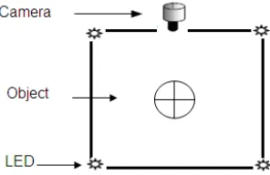
The hypothesis of the PS image capture model is based on four-light PS, which uses a Lambertian diffuse model to describe the surface reflectance properties, with image capture with each under a different positioned illumination. Detailed description and a mathematical foundation of four-lights PS was already introduced. The schematic diagram of four-light PS setup employed in this present study is shown in Figure 4. This (four-light) PS setup was employed to record 2D/3D information of the test objects (i.e. single and multiple 3D hemispheres). The facility was mounted on an optical bench with customised hardware for controlling the directional lighting. The facility included a 8 bit AVT PIKE F100C, colour camera with a resolution of 1 Mega Pixel and images were captured at 20 frames/sec.

Fig. 4. Schematic diagram of the four-light PS experimental setup employed for image capture.

III. PROPOSED NEURAL NETWORK ARCHITECTURE

The human brain is a highly complex non-linear and mas-sively parallel computing system where structures consist of approximately 10 billion basic units called ’the neurons’ and trillions of interconnections. Inspired by the human brain, neural networks emulate the brain’s biological network and their use has been widely established in many applications [20], [21], [22] [23]. NNs have the ability to model non-linear data and subsequently offer a desired output. There are many types of neural network reported in the literature [24], [25], [26]. Multilayer perceptron is a feedforward network [12], where all the connections are from the input to the output. By employing a sufficient number of hidden units (neurons) the network could model any decision boundary with arbitrary accuracy and this concept has been employed herein modelling the bump map of 3D surfaces. The architectural design follows three steps: (i) creating a network, (ii) learning and training algorithms (iii) and testing the network on a dataset. The choice of MLP architecture in implementation is described in the following subsections.

A. MLP network design

(a) (b) (c) (d)

Fig. 5. Test subject (a) 2D Gaussian, (b) network modelled 2D profile, (c) 2D profile with random noise, and (d) network modelled 2D profile.

design was the initial step prior to training and testing for accuracy.

B. Network training

Once the network was created, the next step was training it on a dataset. The data was split into two sets (i.e. training and test) ranging from 60% to 80% depending upon the complexity of the surfaces. The bump map consisted of 1,000 x 1,000 vectors and was divided into regions of 20 x 20 vectors giving 2,500 regions. In the case of modelling a single hemisphere, 60% data allocation for training (1,500 regions) was randomly selected to train the network. For two, three and four adjacent hemispheres 70% of the data, (i.e. 1,750 regions of 20 x 20 points) were chosen for training the network. The training dataset was randomly selected from the whole dataset. Inputs to the network were the data columns corresponding to the position of the pixels and the output represents the predicted value of the gradients of the surface normal vector i.e. tile and slant angle. In the literature, various training algorithms are reported, such as error-back propagation and Levenberg-Marquardt training algorithms. The learning capability of the LMA is reported to be superior [21] and has rapid convergence advantages [29]. Therefore the LMA training algorithm was incorporated to train the network for 12,000 epochs. The stopping principle determines the number of epochs before training of the network is required to be stopped. This usually depends on the sum of the squared errors which are the squared differences between the actual output and the desired output. Training a network involves minimising an error measured across a training dataset which is a function of the weight setting in the MLP. Training is usually carried out until a certain number of epochs (i.e. 12,000 in this case) or the errors decrease to a minimum value where the training could be stopped.

C. Network testing

After the network had been trained on the training dataset, the subsequent step was to test the capability of the network to generate useful outputs. Test data were fed to the network to observe the final output, in order to confirm the actual values. This was achieved by employing the total data minus the training data for testing. For the reported work the designed network employed 5-7 neurons for 2D profile modelling and 24 neurons to model 3D multiple hemispheres.

IV. EXPERIMENTAL PROCEDURE

For a preliminary investigation, a 2D Gaussian as shown Figure 5(a) was a selected for modelling. The proposed network employed 5 neurons to model the profile. The network was trained for 1,200 epochs. For training, 60% data input data were fed to the network. The outputs were plotted to examine how well the network model the 2D Gaussian; the performance is shown in Figure 5(b).

The following step was to include some degree of random noise to modify the underling geometry and to test network modelling capability. The added noise altered the profile as observed in Figure 5(c) The architecture of the network was 7 single layer hidden neurons and 60% data for training the net-work the remaining 40% was kept for testing. The netnet-work was trained for 1,400 epochs. The modelled surface is illustrated in Figure 5(d). Once the network had modelled a curve and 2D

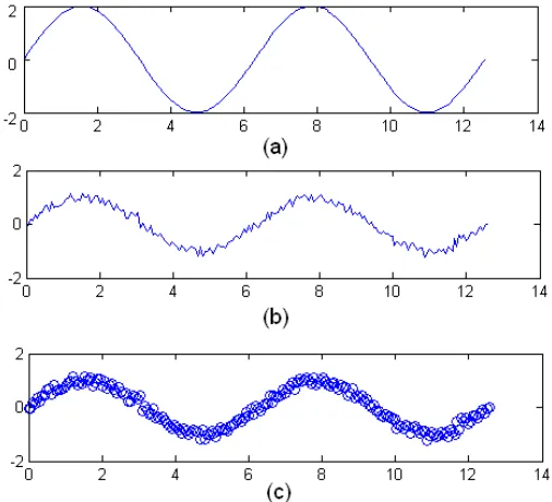
Fig. 6. Test subject (a) sine wave (b) sine wave with added noise, and (c) NN modelled sine wave.

network modelled trajectory is shown in Figure 6.

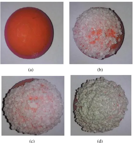
These preliminary results showed that the proposed method could successfully model a 2D profile with noise present. The next step was to employ the proposed method on 3D objects i.e. single axisymmetric hemispheres covered with various level of coarseness ranging from low to medium to as shown in Figure 7.

(a) (b)

(c) (d)

Fig. 7. PS acquired test objects (a) single hemisphere without coarseness, with (b) low level coarseness (c) medium level coarseness, and (d) high level coarseness.

In the following steps, to establish the capability of the proposed model in modelling the non-axisymmetric surfaces, two, three and four adjacent hemisphere were added to the experiments as shown in Figure 8.

The next step was to differentiate between the object and the background (i.e. segmentation). There is a significant difference in terms of gradient; therefore the segmentation process was relatively simple. A threshold value of 5o _for slant and tilt angles was employed to separate the object. The segmented bump map are depicted in Figure 9.

Since four-light sources were employed, four images were captured under different lighting conditions for each of the 3D hemisphere combinations. The data acquisition involved processing four PS images to generate 3D data. Actual surface reconstruction was not the aim here. However, to observe how well the data acquisition performed, a frankot-chellapa reconstruction algorithm [30] was employed for 3D surface reconstruction as shown in Figure 10.

(a) (b)

(c) (d)

Fig. 8. PS acquired test images (a) single hemisphere (b) two adjacent (c) three adjacent and (d) four adjacent hemisphere; all covered with grit to attain coarseness.

(a) (b)

(c) (d)

Fig. 9. Segmented bump map for four set of 3D hemispheres.

(a) (b)

(c) (d)

Fig. 10. Test image 3D reconstruction of single, two, three and four adjacent hemispheres.

was consulted to predict slant and tilt for a given x and y position. At each point on the 3D surface, the network was consulted to predict slant and tilt and the actual slant and tilt was subtracted, giving a measure of surface irregularity. The average irregularities were calculated for the entire set of images.

V. RESULTS

The experiments consisting of a single hemisphere covered with various levels of coarseness, as shown in Figure 7, were chosen for preliminary examination. Depending upon the training algorithm selected and the processor employed, training took a considerable amount of time; however, once the network had been trained it could be rapidly consulted. Training involved the network weights being modified iter-atively to minimise the error between the predicted output gradients and actual gradients. As the training progressed, the error decreased and this as depicted in Figure 11 and this indicated that the training is progressing well.

Fig. 11. NN output error versus epochs. The negative slope indicates that with the increase of epochs the error decreases.

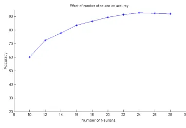
A range of neurons (number varies in between 10 to 28) for a dedicated number of epochs i.e. 12,000, were employed to accomplish the task. For the reported work, the best overall accuracy was achieved via commissioning 24-28 neurons. The

TABLE I

NNPREDICTED SLANT&TILT ANGLES FOR THREE POSITIONS ONx−y AXIS;VALUES ASSOCIATED WITHFIGURE13

Position of gradient onx−yaxis

Actual slant and tilt angles

NN predicted slant and tilt angles

(761,350) 27o_{& 76}o ₂₁o_{& 85}o (761,351) 56o& 37o 61o& 29o

(762,350) 42o_{& 53}o ₃₇o_{& 57}o

best overall accuracy was achieved on employing 24 neurons which is evident in Figure 12.

Fig. 12. Accuracy with the increasing number of neurons.

Once the NN was trained, it was essential to verify that it generalised well. This was achieved by feeding the test data which was hidden from the network during training, into the input layers. To observe the response of the proposed network, three random points on the x−y plane were selected for gradient matching. The position of these three points were (761, 350), (761, 351) and (762, 350), as shown in Figure 13. The two set of gradients, i.e. actual and NN predicted gradients (slant & tilt angles) were matched. Table I illustrates actual and NN predicted gradients for the positions (761, 350), (761, 351) and (762, 350).

In the case of a single 3D hemisphere covered with various levels of coarseness, the network promisingly predicted the gradient of the bump map with overall average deviation (the difference between NN predicted value and actual values) between 3.84o_{to 5.23}o_{(for slant angle) and 4.13}o_{to 7.16}o_(for tilt angle), respectively. Table II illustrates gradients average deviation calculated for test objects. In the case of a single hemisphere, the slight increase in deviation of approximately 2ofor slant and 3ofor tilt angle (from low to high coarseness) is due to the extra level of coarseness added into the surface of the test objects.

The regression analysis was conducted and the MATLAB function POSTREG was used to calculate regression R-value= 0.93, as shown in Figure 14(a) is for Figure 7(d), and confirmed that the network has successfully modelled the underlying symmetry.

Fig. 13. Actual bump map and NN modelling of the surface in terms of the bump map for positions (761, 350), (761, 351) and (762, 350).

TABLE II

NNPREDICTED SLANT&TILT ANGLES AVERAGE ERROR FOR SINGLE3D

HEMISPHERE COVERED WITH GRIT FOR VARIOUS LEVEL OF COARSENESS.

Single hemisphere NN predicted slant an-gles average deviation

NN predicted tilt an-gles average deviation

Without coarseness 3.84o 4.13o Low level coarseness 4.21o _5.75o

Medium level coarseness 4.93o _6.34o

High level coarseness 5.23o _7.16o

objective here was to validate the capability of the network in modelling non-asymmetrical 3D forms, in the presence of noise. This noise was introduced by adding coarseness to the surface of two, three and four adjacent hemispheres. The coarsenesses altered the surface of the objects as observed in Figure 8(d). The proposed method satisfactorily modelled the gradient of the surface normal vector of two adjacent hemispheres with an average deviation of approximately 6.69 o _{for slant angle and 8.51} o _{for tilt angle as shown in Table}

III.

The following step was to model three adjacent non-axisymmetric hemispheres. The network again successfully predicted the desired gradient of the surface normal vec-tor. Finally, a very complex image, i.e. four adjacent non-axisymmetric hemispheres as shown in Figure 8(d), was selected for modelling. The complexity in the shape of the test image was increased; however, the training data was maintained i.e. 70% for training and the remaining 30% for testing. The regression value of R= 0.903 for four hemispheres is shown in Figure 14(b), and confirms its validation. The drop in the regression value was attributed to the surface complexity (in the case of four hemispheres). The network predicted the gradients for four adjacent non-axisymmetric surfaces with average deviation of 9.76o for slant angle and 12.07o for tilt angle. The overall average MLP predicted deviation in slant and tilt angles for the hemispheres consisting of 1, 2, 3 and 4 hemispheres are illustrated in Table III. The slight increase in deviation, for both in slant and tilt angles are due to the asymmetrical complexity in shape for multiple hemispheres.

A synthetically 3D hemisphere and its various combinations as shown in Figure 15 could also be modelled by solving equations. However, mathematically, modelling of more com-plex, irregular and non-axisymmetric 3D surface is extremely challenging. The benefits of the proposed NN based PS approach is that it could model various complex and irregular surfaces such as for instance, a skin lesion as shown in Figure 16 which cannot be simply modelled with equations.

The proposed non-invasive scheme based on a neural net-work and machine vision techniques explored the analysis of surface normal data (tilt and slant angle). It also demonstrated new valuable and potentially complementary 3D indicators in the form of the degree of the 3D surface disruption, which could be employed for skin texture examination. There have been increasing demands for a non-invasive computer vision system which offer benefits such as detailed descriptions of skin. Such a system would be combination is a combination of multi-disciplinary engineering, for instance, computer vision, machine learning, neural networks and texture (skin texture). These systems would be capable of converting qualitative interpretations of the physical and textural characteristics into quantitative results. Subsequently the results could either be translated into a specific suggestion for diagnostic procedures, or to draw judgment over the malignancy of a particular lesion. Currently a diagnosis is often heavily dependent on the clinician experience. Due to the wide range of the diseases, a clear distinction between a melanoma and a benign lesion is very challenging [32]. An alternative solution is that lesion

TABLE III

NNPREDICTED SLANT&TILT ANGLE AVERAGE ERROR FOR NON-AXISYMMETRIC OBJECTS CONSISTING OF1, 2, 3AND4

HEMISPHERES,RESPECTIVELY.

Multiple 3D hemisphere NN predicted slant angle (average error)

NN predicted tilt an-gle (average error)

Single hemisphere 5.23o 7.16o Two adjacent hemisphere 6.69o _8.51o

(a)

(b)

Fig. 14. (a) Slant angle linear regression for single hemisphere with high value of coarseness, (b) Slant angle linear regression for four adjacent hemispheres (high coarseness).

images may be collected (in clinics) at regular intervals and a non-invasive method such as the proposed machine vision based technique could be employed to assist with the early identification of this deadly disease. Therefore, employing a machine vision detection method mainly at primary healthcare could not only help to reduce the number of expensive unnecessary specialists referrals (currently occurring in the NHS), but could assist with more accurate approaches for the identification of melanoma.

VI. CONCLUSION

This article has proposed and demonstrated a novel pho-tometric stereo and MLP neural network based approach for

(a) (b)

(c) (d)

Fig. 15. A computer generated 3D hemispheres.

(a) (b) (c)

Fig. 16. (a) Regular and symmetrical benign lesion, (b) less regular and symmetrical melanoma lesion, (c) an irregular and non-axisymmetric (complex) melanoma.

feature extraction which could subsequently be employed to measure surface irregularities on skin. The PS technique was employed to record 2D/3D data, and the neural network to pre-dict the gradients of the surface normal vectors. The network has initially predicted the gradient for single hemisphere cov-ered with various degree of coarseness, subsequently multiple hemispheres were incorporated to test the performance. Once the proposed network has established its significance the next step of the research is to employ the proposed method on real images and measure skin surface irregularities for objective assessment in the identification of melanoma. Therefore, the following study will discuss the incorporation of medical images analysis.

REFERENCES

[1] L. Lin, X. Ni, L. Zhou, and Z. Qian, “Research on real-time measuring method of dynamic deformation based on machine vision and its application,” Applied Mechanics and Materials, vol. 130, pp. 3572– 3576, 2012.

[2] L. Smith and M. Smith, “Automatic machine vision calibration using statistical and neural network methods,”Image and Vision Computing, vol. 23, no. 10, pp. 887–899, 2005.

[3] L. Gu and Zhou, “Based on the research of the chip electrode positioning system about machine vision in the LED chip automatic measurement,” inIEEE International Conference on Electronics and Optoelectronics, vol. 3, 2011, pp. 120–124.

[4] Y. Ding, L. Smith, M. Smith, and J. Sun, “A computer assisted diagnosis system for malignant melanoma using 3D skin surface texture features and artificial neural network,”International Journal of Modelling, Iden-tification and Control, vol. 9, no. 4, pp. 370–381, 2010.

70, 2009.

[9] Y. Zhou, M. Smith, and L. Smith, “Combinatorial photometric stereo and its application in 3D modelling of melanoma,”Machine Vision and Applications, pp. 1–17, 2011.

[10] C. Research, “Cancer Research UK: cancer statistics key facts-skin[http://info.cancerresearchuk.org/cancerstats],” 2008.

[11] Z. She, Y. Liu, and A. Damatoa, “Combination of features from skin pattern and ABCD analysis for lesion classification,”Skin Research and Technology, vol. 13, no. 1, pp. 25–33, 2007.

[12] I. Aizenberg and C. Moraga, “Multilayer feedforward neural network based on multi-valued neurons (MLMVN) and a backpropagation learn-ing algorithm,”Soft Computing-A Fusion of Foundations, Methodologies and Applications, vol. 11, no. 2, pp. 169–183, 2007.

[13] R. Woodham, “Photometric method for determining surface orientation from multiple images,”Optical Engineering, vol. 19, no. 1, pp. 139–144, 1980.

[14] V. Argyriou and M. Petrou, “Recursive photometric stereo when multiple shadows and highlights are present,” inIEEE Conference on Computer Vision and Pattern Recognition, no. 1, 2010, pp. 1–6.

[15] S. Barsky and M. Petrou, “Surface texture using photometric stereo data: classification and direction of illumination detection,”Journal of Mathematical Imaging and Vision, vol. 29, no. 2, pp. 185–204, 2007. [16] J. Lambert,Photometria sive de mensure de gratibus luminis, colorum

umbrae, 1760.

[17] B. Horn,Robotics Vision. MIT Press, Cambridge, USA, 1986. [18] S. Findlay, N. Shibata, S. Azuma, and Y. Ikuhara, “Prospects for 3D

imaging of dopant atoms in ceramic interfaces.”Journal of Electron Microscopy, vol. 59, pp. S29–S38, 2010.

[19] J. Riphagen, J. Van, and L. Van, “3D surface imaging in medicine: a review of working principles and implications for imaging the unsedated child,”The Journal of Craniofacial Surgery, vol. 19, no. 2, pp. 517–524, 2008.

[20] O. Singh, N. Singla, and M. Sharma, “Optimization of Feedforward neural network for audio classification systems,”International Journal of Advanced Engineering Sciences, vol. 7, no. 1, pp. 98–102, 2011. [21] B. Wilamowski, “Neural network architectures and learning algorithms,”

IEEE Industrial Electronics Magazine, vol. 3, no. 4, pp. 56–63, 2009. [22] S. Anwar, L. Smith, and M. Smith, “3D Texture Analysis using

Co-occurrence Matrix Feature for Classification,” in 4th York Doctoral Conference on Computer Science (YDS11), York, UK, 2011, pp. 05–14. [23] A. Qeethara, “Artificial neural networks in medical diagnosis,” Interna-tional Journal of Computer Science Issues, vol. 8, no. 2, pp. 150–154, 2010.

[24] G. Corsini, M. Diani, and R. Grasso, “Radial Basis Function and Multilayer Perceptron neural networks for sea water optically active parameter estimation in case II waters: a comparison,” International Journal of Remote Sensing, vol. 24, no. 20, pp. 3917–3932, 2003. [25] B. Pandey, S. Ranjan, A. Shukla, and R. Tiwari, “Sentence recognition

using Hopfield neural network,” International Journal of Computer Science Issues, vol. 7, no. 6, pp. 23–26, 2010.

[26] J. Hopfield, “Neural networks and physical systems with emergent collective computational abilities,” in National academy of sciences, vol. 79, no. 8, 1982, p. 2554.

[27] C. Jung, S. Ban, and S. Jeong, “Input and output mapping sensitive auto-associative multilayer perceptron for computer interface system based on image processing of laser pointer spot,”Lecture Notes in Computer Science, vol. 6444, pp. 185–192, 2010.

[28] C. Lee and T. Hsiung, “Sensitivity analysis on a multilayer perceptron model for recognizing liquefaction cases,”Computers and Geotechnics, vol. 36, no. 7, pp. 1157–1163, 2009.

[29] M. Lourakis and A. Argyros, “Is Levenberg-Marquardt the most efficient optimization algorithm for implementing bundle adjustment?” in10th IEEE International Conference on Computer Vision, vol. 2, 2005, pp. 1526–1531.