Expected Sequence Similarity Maximization

Expected Sequence Similarity Maximization

Cyril Allauzen1_{, Shankar Kumar}1_{, Wolfgang Macherey}1_{, Mehryar Mohri}2,1 _{and Michael Riley}1 1_{Google Research, 76 Ninth Avenue, New York, NY 10011}

2_{Courant Institute of Mathematical Sciences, 251 Mercer Street, New York, NY 10012}

Abstract

This paper presents efficient algorithms for expected similarity maximization, which co-incides with minimum Bayes decoding for a similarity-based loss function. Our algorithms are designed for similarity functions that are sequence kernels in a general class of posi-tive definite symmetric kernels. We discuss both a general algorithm and a more efficient algorithm applicable in a common unambigu-ous scenario. We also describe the applica-tion of our algorithms to machine translaapplica-tion and report the results of experiments with sev-eral translation data sets which demonstrate a substantial speed-up. In particular, our results show a speed-up by two orders of magnitude with respect to the original method of Tromble et al. (2008) and by a factor of 3 or more even with respect to an approximate algorithm specifically designed for that task. These re-sults open the path for the exploration of more appropriate or optimal kernels for the specific tasks considered.

1 Introduction

The output of many complex natural language pro-cessing systems such as information extraction, speech recognition, or machine translation systems is a probabilistic automaton. Exploiting the full in-formation provided by this probabilistic automaton can lead to more accurate results than just using the one-best sequence.

Different techniques have been explored in the past to take advantage of the full lattice, some based on the use of a more complex model applied to the automaton as in rescoring, others using addi-tional data or information for reranking the hypothe-ses represented by the automaton. One method for using these probabilistic automata that has been suc-cessful in large-vocabulary speech recognition (Goel and Byrne, 2000) and machine translation (Kumar and Byrne, 2004; Tromble et al., 2008) applications

and that requires no additional data or other com-plex models is the minimum Bayes risk (MBR) de-coding technique. This returns that sequence of the automaton having the minimum expected loss with respect to all sequences accepted by the automaton (Bickel and Doksum, 2001). Often, minimizing the

loss functionLcan be equivalently viewed as

max-imizing a similarity functionK between sequences,

which corresponds to a kernel function when it is positive definite symmetric (Berg et al., 1984). The technique can then be thought of as an expected

se-quence similarity maximization.

This paper considers this expected similarity max-imization view. Since different similarity functions can be used within this framework, one may wish to select the one that is the most appropriate or relevant to the task considered. However, a crucial require-ment for this choice to be realistic is to ensure that for the family of similarity functions considered the expected similarity maximization is efficiently com-putable. Thus, we primarily focus on this algorith-mic problem in this paper, leaving it to future work to study the question of determining how to select the similarity function and report on the benefits of this choice.

A general family of sequence kernels including the sequence kernels used in computational biology, text categorization, spoken-dialog classification, and many other tasks is that of rational kernels (Cortes et al., 2004). We show how the expected similarity maximization can be efficiently computed for these kernels. In section 3, we describe more specifically the framework of expected similarity maximization in the case of rational kernels and the correspond-ing algorithmic problem. In Section 4, we describe both a general method for the computation of the ex-pected similarity maximization, and a more efficient method that can be used with a broad sub-family of rational kernels that verify a condition of non-ambiguity. This latter family includes the class of

n-gram kernels which have been previously used to

apply MBR to machine translation (Tromble et al., 2008). We examine in more detail the use and ap-plication of our algorithms to machine translation in Section 5. Section 6 reports the results of ex-periments applying our algorithms in several large data sets in machine translation. These experiments demonstrate the efficiency of our algorithm which is shown empirically to be two orders of magnitude faster than Tromble et al. (2008) and more than 3 times faster than even an approximation algorithm specifically designed for this problem (Kumar et al., 2009). We start with some preliminary definitions and algorithms related to weighted automata and transducers, following the definitions and terminol-ogy of Cortes et al. (2004).

2 Preliminaries

Weighted transducers are finite-state transducers in

which each transition carries some weight in addi-tion to the input and output labels. The weight set has the structure of a semiring.

A semiring(K,⊕,⊗,0,1)verifies all the axioms

of a ring except from the existence of a negative

el-ement −xfor each x ∈ K, which it may verify or

not. Thus, roughly speaking, a semiring is a ring that may lack negation. It is specified by a set of

values K, two binary operations⊕and⊗, and two

designated values0and1. When⊗is commutative,

the semiring is said to be commutative.

The real semiring (R+,+,×,0,1)is used when

the weights represent probabilities. The log

semiring (R ∪ {−∞,+∞},⊕log,+,∞,0) is

iso-morphic to the real semiring via the

negative-log mapping and is often used in practice

for numerical stability. The tropical semiring

(R∪,{−∞,+∞},min,+,∞,0) is derived from

the log semiring via the Viterbi approximation and is often used in shortest-path applications.

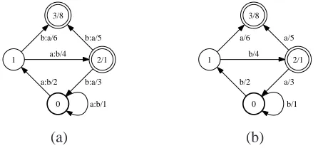
Figure 1(a) shows an example of a weighted finite-state transducer over the real semiring

(R+,+,×,0,1). In this figure, the input and

out-put labels of a transition are separated by a colon delimiter and the weight is indicated after the slash separator. A weighted transducer has a set of initial states represented in the figure by a bold circle and a set of final states, represented by double circles. A path from an initial state to a final state is an accept-ing path.

The weight of an accepting path is obtained by

first ⊗-multiplying the weights of its constituent

0 a:b/1 1

a:b/2

2/1 a:b/4

3/8

b:a/6

b:a/3 b:a/5

0 b/1 1

b/2

2/1 b/4 3/8

a/6

a/3 a/5

(a) (b)

Figure 1: (a) Example of weighted transducerT over the real semiring(R+,+,×,0,1). (b) Example of weighted

automatonA.Acan be obtained fromTby projection on the output andT(aab, bba) =A(bba) = 1×2×6×8 + 2×4×5×8.

transitions and⊗-multiplying this product on the left

by the weight of the initial state of the path (which

equals1in our work) and on the right by the weight

of the final state of the path (displayed after the slash in the figure). The weight associated by a weighted

transducerT to a pair of strings(x, y)∈Σ∗×Σ∗is

denoted byT(x, y)and is obtained by⊕-summing

the weights of all accepting paths with input labelx

and output labely.

For any transducer T, T−1 _{denotes its inverse,}

that is the transducer obtained fromT by swapping

the input and output labels of each transition. For all

x, y∈Σ∗, we haveT−1_{(x, y) =T(y, x).}

The composition of two weighted transducersT1

andT2with matching input and output alphabetsΣ,

is a weighted transducer denoted byT1 ◦T2 when

the semiring is commutative and the sum:

(T1◦T2)(x, y) = X

z∈Σ∗

T1(x, z)⊗T2(z, y) (1)

is well-defined and inK for all x, y (Salomaa and

Soittola, 1978).

Weighted automata can be defined as weighted

transducersAwith identical input and output labels,

for any transition. Since only pairs of the form(x, x)

can have a non-zero weight associated to them by

A, we denote the weight associated byA to(x, x)

by A(x) and call it the weight associated by A to

x. Similarly, in the graph representation of weighted

automata, the output (or input) label is omitted. Fig-ure 1(b) shows an example of a weighted

automa-ton. WhenAandB are weighted automata,A◦B

is called the intersection ofAandB. Omitting the

input labels of a weighted transducerT results in a

weighted automaton which is said to be the output

3 General Framework

LetXbe a probabilistic automaton representing the

output of a complex model for a specific query input. The model may be for example a speech recognition system, an information extraction system, or a ma-chine translation system (which originally motivated our study). For machine translation, the sequences

accepted by X are the potential translations of the

input sentence, each with some probability given by X.

LetΣbe the alphabet for the task considered, e.g.,

words of the target language in machine translation,

and let L: Σ∗ ×Σ∗ → R denote a loss function

defined over the sequences on that alphabet. Given

a reference or hypothesis set H ⊆ Σ∗, minimum

Bayes risk (MBR) decoding consists of selecting a

hypothesisx∈Hwith minimum expected loss with

respect to the probability distributionX(Bickel and

Doksum, 2001; Tromble et al., 2008):

b

x= argmin

x∈H

E

x′_∼X[L(x, x

′_{)]. (2)}

Here, we shall consider the case, frequent in

prac-tice, where minimizing the loss L is equivalent to

maximizing a similarity measureK: Σ∗×Σ∗→R.

When K is a sequence kernel that can be

repre-sented by weighted transducers, it is a rational

ker-nel (Cortes et al., 2004). The problem is then

equiv-alent to the following expected similarity

maximiza-tion:

b

x= argmax

x∈H

E

x′_∼X[K(x, x

′_{)]. (3)}

When K is a positive definite symmetric rational

kernel, it can often be rewritten asK(x, y) = (T ◦

T−1_{)(x, y), where T is a weighted transducer over}

the semiring(R+∪{+∞},+,×,0,1). Equation (3)

can then be rewritten as

b

x= argmax

x∈H

E

x′_∼X[(T ◦T

−1_{)(x, x}′_{)] (4)}

= argmax

x∈H

kA(x)◦T ◦T−1_{◦Xk, (5)}

where we denote by A(x) an automaton accepting

(only) the stringxand byk·kthe sum of the weights

of all accepted paths of a transducer.

4 Algorithms

4.1 General method

Equation (5) could suggest computing A(x)◦T ◦

T−1 _{◦ X for each possible x ∈ H. Instead, we}

can compute a composition based on an

automa-ton accepting all sequences inH,A(H). This leads

to a straightforward method for determining the se-quence maximizing the expected similarity having the following steps:

1. compute the composition X ◦ T, project on

the output and optimize (epsilon-remove,

de-terminize, minimize (Mohri, 2009)) and letY2

be the result;1

2. compute the compositionY1=A(H)◦T;

3. computeY1◦Y2and project on the input, letZ

be the result;2

4. determinizeZ;

5. find the maximum weight path with the label of

that path givingx_b.

While this method can be efficient in various scenar-ios, in some instances the weighted determinization

yieldingZ can be both space- and time-consuming,

even though the input is acyclic. The next two sec-tions describe more efficient algorithms.

Note that in practice, for numerical stability, all of these computations are done in the log semiring

which is isomorphic to(R+∪ {+∞},+,×,0,1). In

particular, the maximum weight path in the last step is then obtained by using a standard single-source shortest-path algorithm.

4.2 Efficient method forn-gram kernels

A common family of rational kernels is the family

ofn-gram kernels. These kernels are widely use as

a similarity measure in natural language processing and computational biology applications, see (Leslie et al., 2002; Lodhi et al., 2002) for instance.

Then-gram kernelKnof ordernis defined as

Kn(x, y) =

X

|z|=n

cx(z)cy(z), (6)

where cx(z) is the number of occurrences of z in

x. Kn is a positive definite symmetric rational

ker-nel since it corresponds to the weighted transducer

Tn ◦Tn−1 where the transducer Tn is defined such

thatTn(x, z) =cx(z)for allx, z ∈Σ∗with|z|=n.

1

Equivalent to computingT−1_{◦X and projecting on the}

input.

2_Z

0 a:ε b:ε

1 a:a

b:b 2

a:a b:b

a:ε b:ε

0

1 a/0.5

2 b/0.5

3 b/1

4 b/1

5 a/1

6 a/1

7 a/0.4

8 b/0.6

b/1

9/1 b/1

a/1

(a) (b)

0

1 a

2 b

3 b

4 b

5 a

6 a

7 a

8 b

b

9 b

a

0

1 a/1

2

b/1 3/1

a/0.2

b/1.5

a/1.8

b/0.5

(c) (d)

ε

a/0 a/0

b/0 b/0

a/0.2

b/1.5

a/1.8 b/0.5

0

1 a/0

2 b/0

3 b/1.5

4 b/0.5

5 a/1.8

6 a/1.8

7 a/0.2

8 b/1.5

b/0.5

9/0 b/1.5

a/1.8

(e) (f)

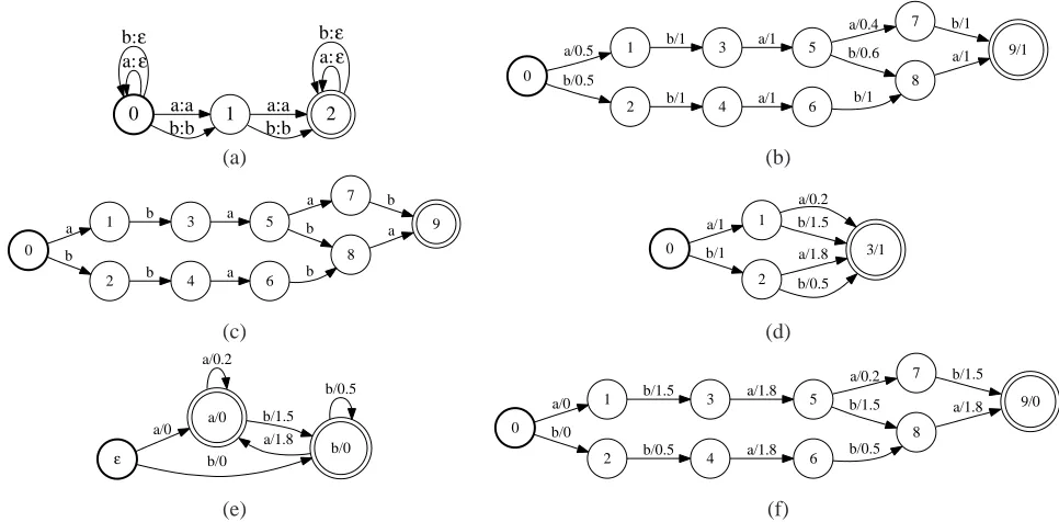
Figure 2: Efficient method for bigram kernel: (a) Counting transducerT2forΣ ={a, b}(over the real semiring). (b)

Probabilistic automatonX(over the real semiring). (c) The hypothesis automatonA(H)(unweighted). (d) Automaton

Y2representing the expected bigram counts inX(over the real semiring). (e) AutomatonY1: the context dependency

model derived fromY2(over the tropical semiring). (f) The compositionA(H)◦Y1(over the tropical semiring).

The transducerT2 forΣ = {a, b} is shown in

Fig-ure 2(a).

Taking advantage of the special structure of n

-gram kernels and of the fact that A(H) is an

un-weighted automaton, we can devise a new and

sig-nificantly more efficient method for computing bx

based on the following steps.

1. Compute the expectedn-gram counts inX: We

compute the compositionX◦T, project on

out-put and optimize (epsilon-remove, determinize,

minimize) and letY2be the result. Observe that

the weighted automatonY2is a compact

repre-sentation of the expectedn-gram counts inX,

i.e. for ann-gramw(i.e.|w|=n):

Y2(w) = X

x∈Σ∗

X(x)cx(w)

= E

x∼X[cx(w)] =cX(w).

(7)

2. Construct a context-dependency model: We

compute the weighted automaton Y1 over the

tropical semiring as follow: the set of states is

Q = {w ∈ Σ∗| |w| ≤ nandwoccurs inX},

the initial state beingǫand every state being

fi-nal; the set of transitionsE contains all 4-tuple

(origin, label, weight, destination) of the form:

• (w, a,0, wa)withwa∈Qand|w| ≤n−

2and

• (aw, b, Y2(awb), wb) with Y2(awb) 6= 0

and|w|=n−2

where a, b ∈ Σ and w ∈ Σ∗. Observe that

w ∈ Q when wa ∈ Q and thataw, wb ∈ Q

whenY2(awb)6= 0. Given a stringx, we have

Y1(x) = X

|w|=n

cX(w)cx(w). (8)

Observe thatY1 is a deterministic automaton,

henceY1(x)can be computed inO(|x|)time.

3. Compute x_b: We compute the composition

A(H)◦Y1.xbis then the label of the accepting

path with the largest weight in this transducer and can be obtained by applying a shortest-path

algorithm to−A(H)◦Y1in the tropical

semir-ing.

The main computational advantage of this method

0 a/1 1 a/c1 2/1 b/c2

0 a 1

2/c1 a

3/c2 b

0 b

1 a

2/c1 a

3/c2

b

b

a b

a

0 b/0

1 a/0

2 a/0

3 b/0

2’/0

b/0 a/0

ε

/c1 3’/0

ε

/c2 b/0

a/0

(a) (b) (c) (d)

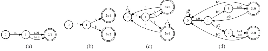
Figure 3: Illustration of the construction ofY1in the unambiguous case. (a) Weighted automatonY2 (over the real

semiring). (b) Deterministic tree automatonY′

2 accepting{aa, ab}(over the tropical semiring). (c) Result of

deter-minization ofΣ∗_Y′

2(over the tropical semiring). (d) Weighted automatonY1(over the tropical semiring).

(+,×) semiring, which can sometimes be costly.

The method has also been shown empirically to be significantly faster than the one described in the pre-vious section.

The algorithm is illustrated in Figure 2. The

al-phabet is Σ = {a, b} and the counting transducer

corresponding to the bigram kernel is given in

Fig-ure 2(a). The evidence probabilistic automaton X

is given in Figure 2(b) and we use as hypothesis set the set of strings that were assigned a non-zero

probability byX; this set is represented by the

deter-ministic finite automatonA(H)given in Figure 2(c).

The result of step 1 of the algorithm is the weighted

automaton Y2 over the real semiring given in

Fig-ure 2(d). The result of step 2 is the weighted

au-tomaton Y1 over the tropical semiring is given in

Figure 2(e). Finally, the result of the composition

A(H)◦Y1 (step 3) is the weighted automaton over

the tropical semiring given in Figure 2(f). The re-sult of the expected similarity maximization is the

string bx = ababa, which is obtained by applying

a shortest-path algorithm to−A(H)◦Y1. Observe

that the stringxwith the largest probability inXis

x=bbabaand is hence different from_bx=ababain this example.

4.3 Efficient method for the unambiguous case

The algorithm presented in the previous section for

n-gram kernels can be generalized to handle a wide

variety of rational kernels.

LetK be an arbitrary rational kernel defined by a

weighted transducerT. LetXT denote the regular

language of the strings output by T. We shall

as-sume thatXT is a finite language, though the results

of this section generalize to the infinite case. Let

Σdenote a new alphabet defined byΣ = {#x:x∈

XT}and consider the simple grammarGof

context-dependent batch rules:

ǫ→#x/x ǫ. (9)

Each such rule inserts the symbol#x immediately

after an occurrencexin the input string. For batch

context-dependent rules, the context of the applica-tion for all rules is determined at once before their application (Kaplan and Kay, 1994). Assume that this grammar is unambiguous for a parallel applica-tion of the rules. This condiapplica-tion means that there is a unique way of parsing an input string using the

strings of XT. The assumption holds for n-gram

sequences, for example, since the rules applicable

are uniquely determined by then-grams (making the

previous section a special case).

Given an acyclic weighted automatonY2over the

tropical semiring accepting a subset ofXT, we can

construct a deterministic weighted automatonY1for

Σ∗L(Y2)when this grammar is unambiguous. The

weight assigned byY1 to an input string is then the

sum of the weights of the substrings accepted byY2.

This can be achieved using weighted determiniza-tion.

This suggests a new method for generalizing Step 2 of the algorithm described in the previous section as follows (see illustration in Figure 3):

(i) use Y2 to construct a deterministic weighted

tree Y₂′ defined on the tropical semiring

ac-cepting the same strings as Y2 with the same

weights, with the final weights equal to the

to-tal weight given by Y2 to the string ending at

that leaf;

(ii) letY1 be the weighted automaton obtained by

first adding self-loops labeled with all elements

of Σ at the initial state ofY₂′ and then

Step (ii) consists of computing a deterministic

weighted automaton for Σ∗Y₂′. This step

corre-sponds to the Aho-Corasick construction (Aho and Corasick, 1975) and can be done in time linear in the size ofY₂′.

This approach assumes that the grammar G of

batch context-dependent rules inferred byXT is

un-ambiguous. This can be tested by constructing the

finite automaton corresponding to all rules inG. The

grammarGis unambiguous iff the resulting

automa-ton is unambiguous (which can be tested using a classical algorithm). An alternative and more ef-ficient test consists of checking the presence of a

failure or default transition to a final state during

the Aho-Corasick construction, which occurs if and only if there is ambiguity.

5 Application to Machine Translation

In machine translation, the BLEU score (Papineni et al., 2001) is typically used as an evaluation metric. In (Tromble et al., 2008), a Minimum Bayes-Risk

decoding approach for MT lattices was introduced.3

The loss function used in that approach was an ap-proximation of the log-BLEU score by a linear

func-tion ofn-gram matches and candidate length. This

loss function corresponds to the following similarity measure:

KLB(x, x′) =θ0|x′|+ X

|w|≤n

θ_|w|cx(w)1x′(w).

(10)

where1x(w)is 1 ifwoccurs inxand 0 otherwise.

(Tromble et al., 2008) implements the MBR de-coder using weighted automata operations. First,

the set of n-grams is extracted from the

lat-tice. Next, the posterior probability p(w|X) of

each n-gram is computed. Starting with the

un-weighted lattice A(H), the contribution of eachn

-gram w to (10) is applied by iteratively

compos-ing with the weighted automaton correspondcompos-ing to

w(w/(θ_|w|p(w|X))w)∗wherew = Σ∗\(Σ∗wΣ∗).

Finally, the MBR hypothesis is extracted as the best path in the automaton. The above steps are carried

out onen-gram at a time. For a moderately large

lat-tice, there can be several thousands ofn-grams and

the procedure becomes expensive. This leads us to investigate methods that do not require processing

then-grams one at a time in order to achieve greater

efficiency.

3

Related approaches were presented in (DeNero et al., 2009; Kumar et al., 2009; Li et al., 2009).

0

1

ε:ε

2

ε:ε

b:ε

3 a:a

a:ε _b:b a:ε b:ε

Figure 4: Transducer T1 over the real semiring for the

alphabet{a, b}.

The first idea is to approximate theKLB

similar-ity measure using a weighted sum of n-gram

ker-nels. This corresponds to approximating1x′(w) by

cx′(w)in (10). This leads us to the following

simi-larity measure:

KN G(x, x′) =θ0|x′|+ X

|w|≤n

θ|w|cx(w)cx′(w)

=θ0|x′|+ X

1≤i≤n

θiKi(x, x′)

(11)

Intuitively, the larger the length ofwthe less likely

it is thatcx(w) 6= 1x(w), which suggests

comput-ing the contribution to KLB(x, x′) of lower-order

n-grams (|w| ≤k) exactly, but using the

approxima-tion byn-gram kernels for the higher-ordern-grams

(|w|> k). This gives the following similarity mea-sure:

K_{N G}k (x, x′) =θ0|x′|+ X

1≤|w|≤k

θ_|w|cx(w)1x′(w)

+ X

k<|w|≤n

θ|w|cx(w)cx′(w)

(12)

Observe thatK0

N G=KN G andKN Gn =KLB.

All these similarity measures can still be com-puted using the framework described in Section 4.

Indeed, there exists a transducer Tn over the real

semiring such thatTn(x, z) = 1x(z)for allx∈Σ∗

andz ∈ Σn_{. The transducerT}

1 for Σ = {a, b}is

given by Figure 4. Let us define the similarity

mea-sureKnas:

Kn(x, x′) = (Tn◦T−

1

n )(x, x′) =

X

|w|=n

cx(w)1x′(w).

(13) Observe that the framework described in Section 4

can still be applied even thoughKnis not

zhen aren

nist02 nist04 nist05 nist06 nist08 nist02 nist04 nist05 nist06 nist08 no mbr 38.7 39.2 38.3 33.5 26.5 64.0 51.8 57.3 45.5 43.8 exact 37.0 39.2 38.6 34.3 27.5 65.2 51.4 58.1 45.2 45.0 approx 39.0 39.9 38.6 34.4 27.4 65.2 52.5 58.1 46.2 45.0 ngram 36.6 39.1 38.1 34.4 27.7 64.3 50.1 56.7 44.1 42.8 ngram1 37.1 39.2 38.5 34.4 27.5 65.2 51.4 58.0 45.2 44.8

Table 1: BLEU score (%)

zhen aren

nist02 nist04 nist05 nist06 nist08 nist02 nist04 nist05 nist06 nist08 exact 3560 7863 5553 6313 5738 12341 23266 11152 11417 11405 approx 168 422 279 335 328 504 1296 528 619 808

ngram 28 72 34 70 43 85 368 105 63 66

ngram1 58 175 96 99 89 368 943 308 167 191

Table 2: MBR Time (in seconds)

can then be expressed as the relevant linear

combi-nation ofKiandKi.

6 Experimental Results

Lattices were generated using a phrase-based MT system similar to the alignment template system de-scribed in (Och and Ney, 2004). Given a source

sen-tence, the system produces a word latticeAthat is a

compact representation of a very largeN-best list of

translation hypotheses for that source sentence and

their likelihoods. The latticeA is converted into a

lattice X that represents a probability distribution

(i.e. the posterior probability distribution given the source sentence) following:

X(x) = P exp(αA(x))

y∈Σ∗exp(αA(y))

(14)

where the scaling factorα∈[0,∞)flattens the

dis-tribution whenα < 1and sharpens it whenα > 1.

We then applied the methods described in Section 5

to the lattice X using as hypothesis set H the

un-weighted lattice obtained fromX.

The following parameters for the n-gram factors

were used:

θ0=

−1

T andθn=

1

4T prn−1 forn≥1. (15)

Experiments were conducted on two language pairs Arabic-English (aren) and Chinese-English (zhen) and for a variety of datasets from the NIST

Open Machine Translation (OpenMT) Evaluation.4

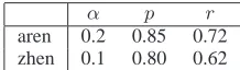
The values ofα,pandrused for each pair are given

4

http://www.nist.gov/speech/tests/mt

α p r

aren 0.2 0.85 0.72

zhen 0.1 0.80 0.62

Table 3: Parameters used for performing MBR.

in Table 3. We used the IBM implementation of the BLEU score (Papineni et al., 2001).

We implemented the following methods using the OpenFst library (Allauzen et al., 2007):

• exact: uses the similarity measureKLB based

on the linearized log-BLEU, implemented as described in (Tromble et al., 2008);

• approx: uses the approximation toKLB from

(Kumar et al., 2009) and described in the ap-pendix;

• ngram: uses the similarity measureKN G

im-plemented using the algorithm of Section 4.2;

• ngram1: uses the similarity measure K1

N G

also implemented using the algorithm of Sec-tion 4.2.

The results from Tables 1-2 show that ngram1

performs as well as exact on all datasets5 _while

be-ing two orders of magnitude faster than exact and overall more than 3 times faster than approx.

7 Conclusion

We showed that for broad families of transducers

T and thus rational kernels, the expected

similar-5

ity maximization problem can be solved efficiently. This opens up the option of seeking the most

appro-priate rational kernel or transducer T for the

spe-cific task considered. In particular, the kernel K

used in our machine translation applications might not be optimal. One may well imagine for

exam-ple that somen-grams should be further emphasized

and others de-emphasized in the definition of the similarity. This can be easily accommodated in the framework of rational kernels by modifying the

tran-sition weights of T. But, ideally, one would wish

to select those weights in an optimal fashion. As mentioned earlier, we leave this question to future work. However, we can offer a brief look at how one could tackle this question. One method for de-termining an optimal kernel for the expected sim-ilarity maximization problem consists of solving a problem similar to that of learning kernels in

classi-fication or regression. LetX1, . . . , Xmbemlattices

with Ref(X1), . . . ,Ref(Xm) the associated

refer-ences and let x_b(K, Xi) be the solution of the

ex-pected similarity maximization for latticeXi when

using kernelK. Then, the kernel learning

optimiza-tion problem can be formulated as follows:

min

K∈K

1

m m

X

i=1

L(x_b(K, Xi),Ref(Xi))

s. t.K =T ◦T−1∧Tr[K]≤C,

whereK is a convex family of rational kernels and

Tr[K] denotes the trace of the kernel matrix. In

particular, we could chooseKas a family of linear

combinations of base rational kernels. Techniques and ideas similar to those discussed by Cortes et al. (2008) for learning sequence kernels could be di-rectly relevant to this problem.

A Appendix

We describe here the approximation of the KLB

similarity measure from Kumar et al. (2009). We

assume in this section that the latticeXis

determin-istic in order to simplify the notations. The posterior

probability ofn-gramwin the latticeXcan be

for-mulated as:

p(w|X) = X

x∈Σ∗

1x(w)P(x|s) =

X

x∈Σ∗

1x(w)X(x)

(16)

where sdenotes the source sentence. When using

the similarity measureKLB defined Equation (10),

Equation (3) can then be reformulated as:

b

x= argmax

x′_∈H

θ0|x′|+ X

w

θ_|w|cx′(w)p(w|X). (17)

The key idea behind this new approximation

algo-rithm is to rewrite then-gram posterior probability

(Equation 16) as follows:

p(w|X) = X

x∈Σ∗

X

e∈EX

f(e, w, πx)X(x) (18)

where EX is the set of transitions of X, πx is

the unique accepting path labeled by x in X and

f(e, w, π)is a score assigned to transitioneon path

πcontainingn-gramw:

f(e, w, π) =   

1 ifw∈e, p(e|X)> p(e′_|X),

ande′_{precedeseonπ}

0 otherwise.

(19)

In other words, for each pathπ, we count the

tran-sition that contributesn-gramwand has the highest

transition posterior probability relative to its

prede-cessors on the pathπ; there is exactly one such

tran-sition on each lattice pathπ.

We note that f(e, w, π) relies on the full path π

which means that it cannot be computed based on local statistics. We therefore approximate the quan-tityf(e, w, π)withf∗_{(e, w, X)that counts the}

tran-sitionewithn-gramwthat has the highest arc

poste-rior probability relative to predecessors in the entire

latticeX.f∗(e, w, X)can be computed locally, and

then-gram posterior probability based onf∗can be

determined as follows:

p(w|G) = X

x∈Σ∗

X

e∈EX

f∗(e, w, X)X(x)

= X

e∈Ex

1w∈ef∗(e, w, X)

X

x∈Σ∗

1πx(e)X(x)

= X

e∈EX

1w∈ef∗(e, w, X)P(e|X),

(20)

whereP(e|X) is the posterior probability of a

lat-tice transition e ∈ EX. The algorithm to perform

Lattice MBR is given in Algorithm 1. For each state

tin the lattice, we maintain a quantity Score(w, t)

for eachn-gramwthat lies on a path from the initial

state tot. Score(w, t)is the highest posterior

prob-ability among all transitions on the paths that

termi-nate ontand containn-gramw. The forward pass

requires computing then-grams introduced by each

transition; to do this, we propagate n-grams (up to

Algorithm 1 MBR Decoding on Lattices

1: Sort the lattice states topologically.

2: Compute backward probabilities of each state. 3: Compute posterior prob. of eachn-gram: 4: for each transitionedo

5: Compute transition posterior probabilityP(e|X). 6: Computen-gram posterior probs.P(w|X): 7: for eachn-gramwintroduced byedo 8: Propagaten−1gram suffix tohe.

9: if p(e|X)>Score(w, T(e)) then 10: Update posterior probs. and scores:

p(w|X)+=p(e|X) −Score(w, T(e)). Score(w, he) =p(e|X).

11: else

12: Score(w, he) =Score(w, T(e)).

13: end if

14: end for 15: end for

16: Assign scores to transitions (given by Equation 17). 17: Find best path in the lattice (Equation 17).

References

Alfred V. Aho and Margaret J. Corasick. 1975. Efficient String Matching: An Aid to Bibliographic Search.

Communications of the ACM, 18(6):333–340.

Cyril Allauzen, Michael Riley, Johan Schalkwyk, Woj-ciech Skut, and Mehryar Mohri. 2007. OpenFst: a general and efficient weighted finite-state transducer library. In CIAA 2007, volume 4783 of LNCS, pages 11–23. Springer. http://www.openfst.org.

Christian Berg, Jens Peter Reus Christensen, and Paul Ressel. 1984. Harmonic Analysis on Semigroups.

Springer-Verlag: Berlin-New York.

Peter J. Bickel and Kjell A. Doksum. 2001.

Mathemati-cal Statistics, vol. I. Prentice Hall.

Corinna Cortes, Patrick Haffner, and Mehryar Mohri. 2004. Rational Kernels: Theory and Algorithms.

Journal of Machine Learning Research, 5:1035–1062.

Corinna Cortes, Mehryar Mohri, and Afshin Ros-tamizadeh. 2008. Learning sequence kernels. In

Pro-ceedings of MLSP 2008, October.

John DeNero, David Chiang, and Kevin Knight. 2009. Fast consensus decoding over translation forests. In

Proceedings of ACL and IJCNLP, pages 567–575.

Vaibhava Goel and William J. Byrne. 2000. Minimum Bayes-risk automatic speech recognition. Computer

Speech and Language, 14(2):115–135.

Ronald M. Kaplan and Martin Kay. 1994. Regular mod-els of phonological rule systems. Computational

Lin-guistics, 20(3).

Philipp Koehn. 2004. Statistical Significance Tests for Machine Translation Evaluation. In EMNLP, Barcelona, Spain.

Shankar Kumar and William J. Byrne. 2004. Minimum Bayes-risk decoding for statistical machine transla-tion. In HLT-NAACL, Boston, MA, USA.

Shankar Kumar, Wolfgang Macherey, Chris Dyer, and Franz Och. 2009. Efficient minimum error rate train-ing and minimum bayes-risk decodtrain-ing for translation hypergraphs and lattices. In Proceedings of the

Asso-ciation for Computational Linguistics and IJCNLP.

Christina S. Leslie, Eleazar Eskin, and William Stafford Noble. 2002. The Spectrum Kernel: A String Kernel for SVM Protein Classification. In Pacific Symposium

on Biocomputing, pages 566–575.

Zhifei Li, Jason Eisner, and Sanjeev Khudanpur. 2009. Variational decoding for statistical machine transla-tion. In Proceedings of ACL and IJCNLP, pages 593– 601.

Huma Lodhi, Craig Saunders, John Shawe-Taylor, Nello Cristianini, and Chris Watskins. 2002. Text classifica-tion using string kernels. Journal of Machine Learning

Research, 2:419–44.

Mehryar Mohri and Richard Sproat. 1996. An Efficient Compiler for Weighted Rewrite Rules. In Proceedings

of ACL ’96, Santa Cruz, California.

Mehryar Mohri. 2009. Weighted automata algorithms. In Manfred Droste, Werner Kuich, and Heiko Vogler, editors, Handbook of Weighted Automata, chapter 6, pages 213–254. Springer.

Franz J. Och and Hermann Ney. 2004. The align-ment template approach to statistical mchine transla-tion. Computational Linguistics, 30(4):417–449. Kishore Papineni, Salim Roukos, Todd Ward, and

Wei-Jing Zhu. 2001. Bleu: a Method for Automatic Evaluation of Machine Translation. Technical Report RC22176 (W0109-022), IBM Research Division. Arto Salomaa and Matti Soittola. 1978.

Automata-Theoretic Aspects of Formal Power Series. Springer.

Roy W. Tromble, Shankar Kumar, Franz J. Och, and Wolfgang Macherey. 2008. Lattice minimum Bayes-risk decoding for statistical machine translation. In

Proceedings of the 2008 Conference on Empirical Methods in Natural Language Processing, pages 620–