Bayesian regression algorithm and its modification with application to public health data

(1)

BAYESIAN REGRESSION ALGORITHM AND ITS MODIFICATION WITH APPLICATION

*1

_{Wan Muhamad Amir W Ahmad,}

1

_{Adam Hussein}

1

_{School of Dental Sciences}

16150

2

_{School of Informatics and Applied Mathematics, Universiti Malaysia Terengganu (UMT), Terengganu Malaysia}

3

_{School of Mathematics Sciences, Universiti Sains Malaysia (USM),}

11800 Minden, Pulau Pinang, Malaysia

ARTICLE INFO ABSTRACT

This paperwork emphasizes an alternative approach of SAS programming language for Linear Bayesian Regression with combination of Fuzzy Regression. The special of this method is, method itself comprises of modeling, bootstrapping for linear minimization programming through fuzzy regression modeling based on the dependent and independent variables.

unrestricted use, distribution, and reproduction in any medium, provided the original work is properly cited.

INTRODUCTION

Multiple linear regression (MLR) analyses are commonly employed in science and non-science fields. The multiple linear regression is given as follows

i i i

i

x

y





0





1 1





2 2





3 3





n

,...

2 ,

1 i



The best-fitting for the regression linear model is by using method of least squares. Least square is the standard approach. The least-squares estimates



0,



1,...,

computed by statistical software. The least square criterion is generalized as follows for general linear regression model









 















n

i

p , i p i

i

x

Y

Q

1

2 1 1 1

1

0



*Corresponding author: Wan Muhamad Amir W Ahmad

School of Dental Sciences, Health Campus,

Malaysia (USM), 16150 Kubang Kerian, Kelantan, Malaysia

ISSN: 0975-833X

Article History:

Received 21st_{March, 2017}

Received in revised form 10th_{April, 2017}

Accepted 09th_{May, 2017}

Published online 30th_{June, 2017}

Citation: Wan Muhamad Amir W Ahmad, Nor Azlida Aleng, Zalila Ali, Ruhaya Hasan, Adam Hussein

“Bayesian regression algorithm and its modification with application to public health data

Key words:

Bootstrap, Linear Regression.

Available online at http://www.journal

REVEIW ARTICLE

BAYESIAN REGRESSION ALGORITHM AND ITS MODIFICATION WITH APPLICATION

TO PUBLIC HEALTH DATA

Wan Muhamad Amir W Ahmad,

2

_{Nor Azlida Aleng,}

3

_{Zalila Ali,}

1

Adam Hussein

and

2

_{Nurfadhlina Abdul Halim}

School of Dental Sciences, Health Campus, Universiti Sains Malaysia (USM),

16150 Kubang Kerian, Kelantan, Malaysia

School of Informatics and Applied Mathematics, Universiti Malaysia Terengganu (UMT), Terengganu Malaysia

School of Mathematics Sciences, Universiti Sains Malaysia (USM),

11800 Minden, Pulau Pinang, Malaysia

ABSTRACT

This paperwork emphasizes an alternative approach of SAS programming language for Linear Bayesian Regression with combination of Fuzzy Regression. The special of this method is, method itself comprises of modeling, bootstrapping for linear minimization programming through fuzzy regression modeling based on the dependent and independent variables.

et al. Thisis an open access article distributed under the Creative Commons Att use, distribution, and reproduction in any medium, provided the original work is properly cited.

Multiple linear regression (MLR) analyses are commonly science fields. The multiple

fitting for the regression linear model is by using . Least square is the standard approach.

n



are usually computed by statistical software. The least square criterion is generalized as follows for general linear regression model

*Corresponding author: Wan Muhamad Amir W Ahmad

School of Dental Sciences, Health Campus, Universiti Sains 16150 Kubang Kerian, Kelantan, Malaysia

The least square estimator are those values of

that minimize Q. let us denote the vector of the least square estimate regression coefficient

1





p

  

 

  

 

  

1 0

p 

The least square normal equations for the general linear regression model are given as follow

Y

X









And the least square estimator are:



 



1 p p p

1

1 p

Y

X

 











The method of maximum likelihood leads to the same estimators for normal error regression model

International Journal of Current Research

Vol. 9, Issue, 06, pp.53088-53094, June, 2017

Wan Muhamad Amir W Ahmad, Nor Azlida Aleng, Zalila Ali, Ruhaya Hasan, Adam Husseinand Nurfadhlina Abdul Halim

Bayesian regression algorithm and its modification with application to public health data”, International Journal of Current Research

Available online at http://www.journalcra.com

z

BAYESIAN REGRESSION ALGORITHM AND ITS MODIFICATION WITH APPLICATION

1

_{Ruhaya Hasan,}

Universiti Sains Malaysia (USM),

School of Informatics and Applied Mathematics, Universiti Malaysia Terengganu (UMT), Terengganu Malaysia

School of Mathematics Sciences, Universiti Sains Malaysia (USM),

This paperwork emphasizes an alternative approach of SAS programming language for Linear Bayesian Regression with combination of Fuzzy Regression. The special of this method is, the method itself comprises of modeling, bootstrapping for linear minimization programming through fuzzy regression modeling based on the dependent and independent variables.

is an open access article distributed under the Creative Commons Attribution License, which permits

The least square estimator are those values of



0,



1,...,



p1

. let us denote the vector of the least square estimate regression coefficient



₀,



₁,...,



_p_₁ as b:

The least square normal equations for the general linear regression model are given as follow

And the least square estimator are:

The method of maximum likelihood leads to the same estimators for normal error regression model

1 n 1 p p n 1

n

Y





X





_





 INTERNATIONAL JOURNAL

OF CURRENT RESEARCH

and Nurfadhlina Abdul Halim. 2017.

(2)

as those obtained by the method of least square



 



1 p p p 1 1 p

Y

X

   







.

The bootstrap method starts with an original sample which is taken from the considered specific population. The next step is to duplicates the original sample in a number of times to create a new population regard to original population. In that case, the bootstrap draws several samples with replacement by random sampling approach, and as a result it provides a different sample from the original sample. This technique stores the new set of data and creating a new distribution for further analysis. (Efron et al., 1993; Higgins, 2005). The advantage of using bootstrap is its ability to develop a sample the same size of the original, which may include an observation several times while omitting other observations.

Fuzzy regression be written as ,

with the explanation variables are assumed to be precise. Our aim is to estimate these parameters (Amir et. al, 2016). In this case, are assumed as symmetric fuzzy numbers which can be presented by intervals. In fuzzy regression methodology, parameters are estimated by minimising total vagueness in the model.

.Using ,it can be written

(Amir et. al, 2016).

represents radius and cannot be negative, therefore, on the

right-hand side of equation ,

absolute values of are taken. Suppose there m data point, each comprising vector (Amir et. al, 2016). Then

parameters are estimated by minimising the quantity, which is total vagueness of the model-data set combination, subject to the constraint that each data point must fall within estimated value of response variable. This can be visualized as the following linear programming problem, minimised

and subject to

and

.

and . Simple procedure is commonly used to solve the linear programming problem. (Kacprzyk and Fedrizzi, 1992). Data for this study is a sample which is composed of four variables(Amir et. al, 2016)

Sample Size Determination

Sample size for multiple regression analysis were calculated by using G*power with effect size = 0.35, 0.05, power of the study = 0.90 and number of predictor were 4. The minimum sample size requires is 50 respondents.

Analysis: A priori: Compute required sample size

Input: Effect size f² = 0.35 α err prob = 0.05

Power (1-β err prob) = 0.90 Number of predictors = 4

[image:2.595.311.514.52.237.2]

Output: Noncentrality parameter λ=17.5000 Critical F = 2.5787 Numerator, df. = 4 Denominator, df. = 45 Total sample size = 50 Actual power = 0.90

Table 1. Description of Cholesterol Data

Num. Variables Explanation of user variables 1. Choltot Total Cholesterol

2. Hdl HDL Cholesterol 3 Trig Triglycerides 4 Waist Waist circumferences

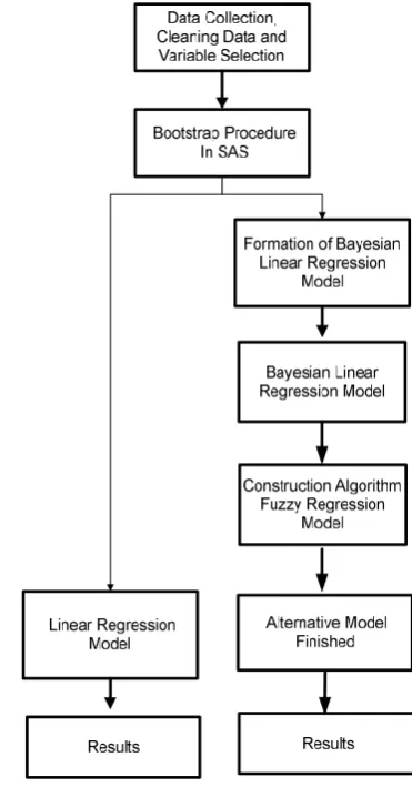
[image:2.595.331.517.296.651.2]

Algorithm and Flow Chart for Modified Bayesian Linear Regression Analysis Method

Figure 1. Modified Bayesian Linear Regression Analysis

/*ADDING BOOTSTRAPPING ALGORITHM TO THE METHOD */

%MACRO bootstrap(data=_last_, booted=booted, boots=2, seed=1234);

DATA &booted;

** randomly picks an integer from 1 to n;

pickobs = INT(RANUNI(&seed)*n)+1; k kx Z x Z x Z Z

Y 0 1 1 2 2

s

x

i

'

s

Z_i'

kj k j

j

j Z Zx Z x Z x

y  0 1 1  2 2  

 c w

i a a

Z 1, 1 yja0c,a0w

  

a1c,a1w x1j  anc,anwxnj

y

_jw

nj nw j

w w

jw a a x a x

y  0  1 1 

ij

x



n



row

a 1

i Z







    m j nj nw j w

w a x a x

a 1 1 1 0  j n i ij iw w n i ij ic

c a x a a x Y

a                      



  1 0 1 0 j n i ij iw w n i ij ic

c a x a a x Y

a                      



  1 0 1 0 0  iw a

(3)

** POINT tells SAS to read value pickobs ** NOBS sets n to number of obs in &Data;

** when the point option is used SAS will loop through the data step forever;

SET &data POINT = pickobs NOBS = n; ** saves number of current bootstrap;

REPLICATE=int(i/n)+1; i+1;

** stop will leave data set when n*&boots obs have been created;

IF i > n*&boots THEN STOP; RUN;

%MEND bootstrap;

Data Cholesterol;

Input choltot Hdl Trig Waist;

Cards;

1814676 98.0 22039151 94.0 22039151 94.0 21345123 95.0 17942139 81.0 17942139 81.0 1144262104.0 1144262104.0 26771122 91.5 26771122 91.5 2357391 96.5 2475585 92.0 19957126116.5 19957126116.5 16245100 88.0 23770222 91.5 2076681 85.0 20249118106.5 1844398 90.0 29956207113.0 18447118 95.0 1819271 97.5 22039151 94.0 22039151 94.0 1804758 97.0 17942139 81.0 17942139 81.0 17942139 81.0 17942139 81.0 1144262104.0 1144262104.0 1144262104.0 2475585 92.0 19957126116.5 19957126116.5 16245100 88.0 21032193 95.5 23770222 91.5 2076681 85.0 20249118106.5 29956207113.0 18447118 95.0 ;

odsrtffile='abc.rtf'style=journal;

**generate bootstrap sample;

%bootstrap(data=Cholesterol, boots=2);

run;

/*PRINT DATA */

procprintdata=booted;

run;

odsrtfclose;

/* LINEAR REGRESSION MODELING AND RESIDUAL NORMALITY CHECKING*/

Data Booted;

Input choltotbayes hdl trig waist;

Cards;

207.5473.0091.00 96.50 190.9445.00123.00 95.00 193.4066.0081.00 85.00 202.9942.00139.00 81.00 207.5473.0091.00 96.50 190.9445.00123.00 95.00 203.4739.00151.00 94.00 202.9942.00139.00 81.00 170.8143.0098.00 90.00 137.8642.0062.00104.00 203.4739.00151.00 94.00 264.4856.00207.00113.00 190.9445.00123.00 95.00 193.4066.0081.00 85.00 264.4856.00207.00113.00 137.8642.0062.00104.00 193.4066.0081.00 85.00 303.1270.00222.00 91.50 204.0057.00126.00116.50 220.1192.0071.00 97.50 178.0355.0085.00 92.00 175.8845.00100.00 88.00 207.5473.0091.00 96.50 170.8143.0098.00 90.00 202.9942.00139.00 81.00 137.8642.0062.00104.00 156.1546.0076.00 98.00 220.1192.0071.00 97.50 193.4066.0081.00 85.00 229.4871.00122.00 91.50 204.0057.00126.00116.50 137.8642.0062.00104.00 202.9942.00139.00 81.00 203.4739.00151.00 94.00 202.9942.00139.00 81.00 178.0355.0085.00 92.00 203.4739.00151.00 94.00 190.1247.00118.00 95.00 203.4739.00151.00 94.00 189.4149.00118.00106.50 190.1247.00118.00 95.00 189.4149.00118.00106.50 137.8642.0062.00104.00 175.8845.00100.00 88.00 137.8642.0062.00104.00 224.2632.00193.00 95.50 202.9942.00139.00 81.00 204.0057.00126.00116.50 264.4856.00207.00113.00 144.4247.0058.00 97.00 204.0057.00126.00116.50 202.9942.00139.00 81.00 203.4739.00151.00 94.00 137.8642.0062.00104.00 202.9942.00139.00 81.00 207.5473.0091.00 96.50 175.8845.00100.00 88.00 178.0355.0085.00 92.00 137.8642.0062.00104.00 193.4066.0081.00 85.00 202.9942.00139.00 81.00 137.8642.0062.00104.00

(4)

203.4739.00151.00 94.00 137.8642.0062.00104.00 175.8845.00100.00 88.00 175.8845.00100.00 88.00 220.1192.0071.00 97.50 137.8642.0062.00104.00 170.8143.0098.00 90.00 137.8642.0062.00104.00 204.0057.00126.00116.50 137.8642.0062.00104.00 137.8642.0062.00104.00 220.1192.0071.00 97.50 193.4066.0081.00 85.00 193.4066.0081.00 85.00 178.0355.0085.00 92.00 144.4247.0058.00 97.00 204.0057.00126.00116.50 204.0057.00126.00116.50 204.0057.00126.00116.50 303.1270.00222.00 91.50 203.4739.00151.00 94.00 190.1247.00118.00 95.00

run;

Odsrtffile='abc.rtf'style=journal;

odsgraphicson;

procregdata=Booted plots=all;

model choltotbayes = hdl trig waist/p ;

run;

odsgraphicsoff;

odsrtfclose;

run;

/* BAYESIAN REGRESSION MODEL*/

Data Booted;

Input choltotbayesian hdl trig waist;

Cards;

207.5473.0091.00 96.50 190.9445.00123.00 95.00 193.4066.0081.00 85.00 202.9942.00139.00 81.00 207.5473.0091.00 96.50 190.9445.00123.00 95.00 203.4739.00151.00 94.00 202.9942.00139.00 81.00 170.8143.0098.00 90.00 137.8642.0062.00104.00 203.4739.00151.00 94.00 264.4856.00207.00113.00 190.9445.00123.00 95.00 193.4066.0081.00 85.00 264.4856.00207.00113.00 137.8642.0062.00104.00 193.4066.0081.00 85.00 303.1270.00222.00 91.50 204.0057.00126.00116.50 220.1192.0071.00 97.50 178.0355.0085.00 92.00 175.8845.00100.00 88.00 207.5473.0091.00 96.50 170.8143.0098.00 90.00 202.9942.00139.00 81.00 137.8642.0062.00104.00 156.1546.0076.00 98.00 220.1192.0071.00 97.50 193.4066.0081.00 85.00 229.4871.00122.00 91.50 204.0057.00126.00116.50 137.8642.0062.00104.00 202.9942.00139.00 81.00 203.4739.00151.00 94.00

202.9942.00139.00 81.00 178.0355.0085.00 92.00 203.4739.00151.00 94.00 190.1247.00118.00 95.00 203.4739.00151.00 94.00 189.4149.00118.00106.50 190.1247.00118.00 95.00 189.4149.00118.00106.50 137.8642.0062.00104.00 175.8845.00100.00 88.00 137.8642.0062.00104.00 224.2632.00193.00 95.50 202.9942.00139.00 81.00 204.0057.00126.00116.50 264.4856.00207.00113.00 144.4247.0058.00 97.00 204.0057.00126.00116.50 202.9942.00139.00 81.00 203.4739.00151.00 94.00 137.8642.0062.00104.00 202.9942.00139.00 81.00 207.5473.0091.00 96.50 175.8845.00100.00 88.00 178.0355.0085.00 92.00 137.8642.0062.00104.00 193.4066.0081.00 85.00 202.9942.00139.00 81.00 137.8642.0062.00104.00 203.4739.00151.00 94.00 137.8642.0062.00104.00 175.8845.00100.00 88.00 175.8845.00100.00 88.00 220.1192.0071.00 97.50 137.8642.0062.00104.00 170.8143.0098.00 90.00 137.8642.0062.00104.00 204.0057.00126.00116.50 137.8642.0062.00104.00 137.8642.0062.00104.00 220.1192.0071.00 97.50 193.4066.0081.00 85.00 193.4066.0081.00 85.00 178.0355.0085.00 92.00 144.4247.0058.00 97.00 204.0057.00126.00116.50 204.0057.00126.00116.50 204.0057.00126.00116.50 303.1270.00222.00 91.50 203.4739.00151.00 94.00 190.1247.00118.00 95.00

;

run;

odsrtffile='abc.rtf'style=journal;

odsgraphicson;

procgenmoddata=Booted;

model choltotbayesian = hdl trig waist / dist=normal

link=identity;

bayesseed=1OutPost=Post diagnostics=allsummary=all;;

run;

odsgraphicsoff;

odsrtfclose;

run;

/* BAYESIAN FUZZY REGRESSION*/

Title ‘Linear programming’;

data plant;

input choltotbayesian hdl trig waist;

datalines;

(5)

207.5473.0091.00 96.50 190.9445.00123.00 95.00 193.4066.0081.00 85.00 202.9942.00139.00 81.00 207.5473.0091.00 96.50 190.9445.00123.00 95.00 203.4739.00151.00 94.00 202.9942.00139.00 81.00 170.8143.0098.00 90.00 137.8642.0062.00104.00 203.4739.00151.00 94.00 264.4856.00207.00113.00 190.9445.00123.00 95.00 193.4066.0081.00 85.00 264.4856.00207.00113.00 137.8642.0062.00104.00 193.4066.0081.00 85.00 303.1270.00222.00 91.50 204.0057.00126.00116.50 220.1192.0071.00 97.50 178.0355.0085.00 92.00 175.8845.00100.00 88.00 207.5473.0091.00 96.50 170.8143.0098.00 90.00 202.9942.00139.00 81.00 137.8642.0062.00104.00 156.1546.0076.00 98.00 220.1192.0071.00 97.50 193.4066.0081.00 85.00 229.4871.00122.00 91.50 204.0057.00126.00116.50 137.8642.0062.00104.00 202.9942.00139.00 81.00 203.4739.00151.00 94.00 202.9942.00139.00 81.00 178.0355.0085.00 92.00 203.4739.00151.00 94.00 190.1247.00118.00 95.00 203.4739.00151.00 94.00 189.4149.00118.00106.50 190.1247.00118.00 95.00 189.4149.00118.00106.50 137.8642.0062.00104.00 175.8845.00100.00 88.00 137.8642.0062.00104.00 224.2632.00193.00 95.50 202.9942.00139.00 81.00 204.0057.00126.00116.50 264.4856.00207.00113.00 144.4247.0058.00 97.00 204.0057.00126.00116.50 202.9942.00139.00 81.00 203.4739.00151.00 94.00 137.8642.0062.00104.00 202.9942.00139.00 81.00 207.5473.0091.00 96.50 175.8845.00100.00 88.00 178.0355.0085.00 92.00 137.8642.0062.00104.00 193.4066.0081.00 85.00 202.9942.00139.00 81.00 137.8642.0062.00104.00 203.4739.00151.00 94.00 137.8642.0062.00104.00 175.8845.00100.00 88.00 175.8845.00100.00 88.00 220.1192.0071.00 97.50 137.8642.0062.00104.00 170.8143.0098.00 90.00 137.8642.0062.00104.00 204.0057.00126.00116.50 137.8642.0062.00104.00 137.8642.0062.00104.00

220.1192.0071.00 97.50 193.4066.0081.00 85.00 193.4066.0081.00 85.00 178.0355.0085.00 92.00 144.4247.0058.00 97.00 204.0057.00126.00116.50 204.0057.00126.00116.50 204.0057.00126.00116.50 303.1270.00222.00 91.50 203.4739.00151.00 94.00 190.1247.00118.00 95.00

;

run;

odsrtffile='result_ex1.rtf' ;

procoptmodel; set j= 1..84;

number choltotbayesian{j}, hdl{j}, trig{j} waist{j};

readdata plant into [_n_]choltotbayesian hdl trig waist;

/*Print choltotbayesian hdl trig waist*/

print choltotbayesian hdl trig waist;

number n init8;

/*Total number of Observations*/ /*Decision Variables*/

var aw{1..4}>=0;

/*Theses four variables are bounded*/

var ac{1..4};

/* These four variables are not bounded*/

/* Objective function*/

min z1= aw[1] * n + sum{i in j} hdl[i] * aw[2] + sum{i in j} trig[i] * aw[3]+ sum{i in j} waist[i] * aw[4];

/*Linear Constraints*/

con c{i in 1..n}:

ac[1]+hdl[i]*ac[2]+trig[i]*ac[3]+waist[i]*ac[4]-aw[1

]-hdl[i]*aw[2]- trig[i]*aw[3]- waist[i]*aw[4] <= choltotbayesian[i];

con c1{i in 1..n}:

ac[1]+hdl[i]*ac[2]+trig[i]*ac[3]+waist[i]*ac[4] +aw[1]+ hdl[i]*aw[2]+trig[i]*aw[3]+waist[i]*aw[4] >= choltotbayesian[i];

expand; /* This provides all equations */

solve;

print ac aw;

quit;

ods rtf close;

RESULTS

[image:5.595.320.547.715.800.2]

Part I: Results from Bayesian Multiple linear Regression

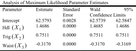
Table 3. Results from Bayesian Multiple linear Regression

Analysis of Maximum Likelihood Parameter Estimates Parameter Estimate Standard

Error

Wald 95% Confidence Limits Intercept 62.5793 0.0028 62.5739 62.5847 Hdl (X₁) 1.4686 0.0000 1.4685 1.4686 Trig(X₂) 0.7511 0.0000 0.7511 0.7511 Waist(X₃) -0.3170 0.0000 -0.3170 -0.3169

(6)

With Choltotbayesian(Y)

Multiple Bayesian Linear Regression (MBLR) is given as follows:

)

(Y = 62.5793 + 1.4686 (X₁) + 0.7511 (X₂)

-0.3170(X₃)

where

(X₁)is High Density Lipoprotein reading (X₂)is a Triglycerides reading

[image:6.595.39.289.210.568.2]

(X₃)is Waist reading

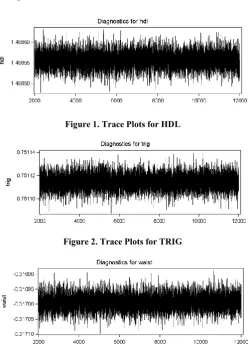
[image:6.595.346.520.256.383.2]

Figure 1. Trace Plots for HDL

Figure 2. Trace Plots for TRIG

Figure 3. Trace Plots for Intercept

We also can assess convergence by visualization examination through trace plot. Trace plot consist of the plot sampled values of a parameter versus the sample number. Figure 1.1 till Figure 1.3 summarize the result of trace plot of our finding. The Figure 1.1, 1.2 and 1.3 shows the behaviour of the trace plots. From the plot, we can see that all parameters have relatively good mixing properties. Good mixing of the chain indicate that we can get the good results and the samples stay close to the high-density region of the target distribution.

Fitted Bayesian Multiple Linear Regression with standard error is given as follows:

)

(Y = 62.5793 + 1.4686 (X1) + 0.7511 (X2)

Std. Error (0.0028) (0.0000) (0.0000)

-0.3170(X₃) ……….…………..… (2.1)

Std. error (0.0000)

Upper or lower limits of prediction interval are computed from the prediction equation (2.1) by taking the coefficient as their corresponding estimated values plus or minus standard error.

Upper limits

)

(Y = 62.5821 + 1.4686 (X₁) + 0.7511 (X₂)

-0.3170 (x₃)….………....……(2.2)

Lowerlimits

)

(Y = 62.5765 + 1.4686 (x₁) + 0.7511 (x₂)

-0.3170 (x3)….………....(2.3)

Lower limit Upper limit Width 207.544

190.934 193.398 202.984 207.544 190.934 203.470

207.550 190.939 193.404 202.989 207.550 190.939 203.476

.0056 .0056 .0056 .0056 .0056 .0056 .0056



303.117 203.470 190.116

303.123 203.476 190.121

.0056 .0056 .0056 Average width 0.0056

Part II: Results From Fitted Model For Fuzzy

Regression

Table 4. Value of centre (AC) and radius (AW)

[1] ac aw 1 62.65633 0.0015848 2 1.46796 0.0000000 3 0.75085 0.0000000 4 -0.31716 0.0000000

Fitted model for fuzzy regression (FR) for

Choltotbayesian(Y)= <62.65633, 0.0015848> + < 1.46796, 0.0000000> Hdl + <0.75085, 0.0000000> Trig +

<-0.31716, 0.0000000> Waist ……….(2.4)

Upper or lower limits of prediction intervals are computed from the prediction equation (2.4) by taking the coefficient as their corresponding estimated values plus or minus standard error.

Upper limits

Y= <62.6547452> + < 1.46796, 0> (X₁) +

<0.75085, 0> (X₂) +< -0.31716, 0> (X₃)…….(2.5)

Lowers limits

Y= <62.6579148> + < 1.46796, 0> (X₁) +

<0.75085, 0> (X2) +<-0.31716, 0> (X3)…….(2.6)

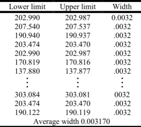
[image:6.595.365.498.452.507.2]

(7)

Lower limit Upper limit Width 202.990

207.540 190.940 203.474 202.990 170.819 137.880

202.987 207.537 190.937 203.470 202.987 170.816 137.877

0.0032 .0032 .0032 .0032 .0032 .0032 .0032



303.084 203.474 190.122

303.081 203.470 190.119

0032 .0032 .0032 Average width 0.003170

The width of prediction intervals with respect to bayesian multiple linear regression model and bayesian fuzzy regression model corresponding to each set of observed explanatory variables is computed in SPSS and the results are reported in Table 4. From this table, the average width for former was found to be 0.005600, while that of the latter was only 0.003170, thereby indicating the superiority of fuzzy regression methodology.

SUMMARY AND DISCUSSION

This paper presents an algorithm and illustrated the procedure of modeling by using modified Bayesian linear regression through SAS language. Our aim is to share the algorithm and also provide the researcher with an alternative programming that suitable for a small sample size. This proposed method can be applied to small sample size data, especially when limited data is obtained for example in public health.

Acknowledgements

The authors would like to express their gratitude to Universiti Sains Malaysia (USM) for providing the research funding (Grant no.304/PPSG/61313187, School of Dental Sciences)

REFERENCES

Amir, Wan Muhamad; Shafiq, Mohamad; A.Rahim, Hanafi; Liza, Puspa; Aleng, Azlida; and Abdullah, Zailani, 2016. "Algorithm for Combining Robust and Bootstrap In Multiple Linear Model Regression (SAS)," Journal of Modern Applied Statistical Methods: Vol. 15: Iss. 1, Article 46

Amir, Wan Muhamad; Shafiq, Mohamad; Mokhtar, Kasypi; Aleng, Nor Azlida; A.Rahim, Hanafi; and Ali, Zalila 2016. "Simple Response Surface Methodology Using RSREG (SAS)," Journal of Modern Applied Statistical Methods: Vol. 15: Iss. 1, Article 44.

Efron, Bradley and Robert J. Tibshirani. 1993. An Introduction to the Bootstrap. New York, NY: Chapman and Hall.

Higgins, G. E. 2005.Statistical Significance Testing: The Bootstrapping Method and an Application to Self-Control Theory. The Southwest Journal of Criminal Justice. Vol 2(1).pp 54-76

Kacprzyk J. and Fedrizzi M. 1992. Fuzzy Regression Analysis, Omnitech Press, Warsaw.

Lambert, D. 1992. ZIP with an application to defects in manufacturing. Journal of Technometrics, 34, 1-14. Zafakali, Nur Syabiha binti and Ahmad, Wan Muhamad Amir

bin W 2013. "Modeling and Handling Overdispersion Health Science Data with Zero-Inflated Poisson Model," Journal of Modern Applied Statistical Methods: Vol. 12: Iss. 1, Article 28.

*******

[image:7.595.89.235.54.185.2]