Why the Speed of Light Is Not a Constant
Paul Smeulders Sutton Courtenay, UK Email: [email protected]
Received February 12,2012; revised March 16, 2012; accepted March 25, 2012
ABSTRACT
A variable Speed of Light is supported by the fact that all direct measurements of that speed are basically flawed, be- cause the “meter per second” is proportional to the Speed of Light. Since it is impossible to measure the Speed of Light directly, any variations of it can only be obtained in an indirect way. It will be shown that the recent Supernovae data are in very good agreement with a universe that is slowly expanding exponentially with a Speed of Light that falls over time, inversely proportionally to the expansion of the universe. It will be shown that the definition of the angular and standard impulse momentum has to be modified to get a consistent expansion of the universe. And that all clocks run inversely proportionally to the red-shift z + 1. General Relativity remains valid even with a varying Speed of Light and also Quantum Mechanics is unaffected.
Keywords: Variable Speed of Light; Expansion of Universe; Conservation of Energy and Angular Impulse Momentum;
Supernovae
1. Introduction
It is essential that when making a measurement to make sure that the two quantities involved are independent of each other. When the two quantities are shown to be pro- portional to each other, one always obtains a constant value [1]. It was shown that the “m/s” is proportionally to the speed of the electron going around the proton. The latter speed equals the fine-structure constant α times the speed of light. K. Webb et al. [2] have shown that α only changes little over most of the time of the visible uni- verse. Hence measurements of Speed of Light are basi- cally flawed and invalid.
There have been several publications in the past deal- ing with Variable Speed of Light (VSL) in cosmology [3-6]. Some of the models conserve the mass of the uni- verse and therefore not the energy. And all let the value of the speed of light vary in m/s. The VSL scheme dis- cussed in this paper will conserve the energy throughout. Angular impulse momentum and impulse momentum will also be conserved, but with some modification in the definition of these quantities in an expanding universe (this has to be done in any case!). And the measured value of the speed of light is constant. So the apparent speed of light is constant!
It will be shown in Section 2, that the Hubble Law fits the Supernovae data in an excellent way when a varying Speed of light is taken into account. This then automati- cally leads to a slowly expanding universe, with an ex- pansion that is exponentially in time. Such an expansion
is structurally very different from a power scaled model [7] leading to a very different universe. Although for small red-shifts the exponential expansion follows a power scaling a(t) = (t/t0)n with n = 1/2 when c(t) = c0/a(t) and n
= 1 in case c is really constant in time. A power scaling would then lead to a very dense universe (ρ > ρcr) in the
case of the VSL and an empty universe for a constant speed of light.
Section 3 will demonstrate that the present definition of the angular impulse momentum leads to orbits that are not proportional to the expansion of the universe and that in order to make a consistent expansion one has to multi- ply the angular momentum with z + 1. Then any orbit, including electrons around protons, will scale with a(t).
In Section 4, it is shown that any clock scales inversely proportional to z + 1. All processes will therefore run faster when going back in time. It is also shown that the Lorentz length scales with a(t) and therefore Relativity remains valid even for a changing Speed of Light.
2. The Hubble Law
curve that can be explained by an expanding empty uni- verse or also by a flat dark energy model [8].
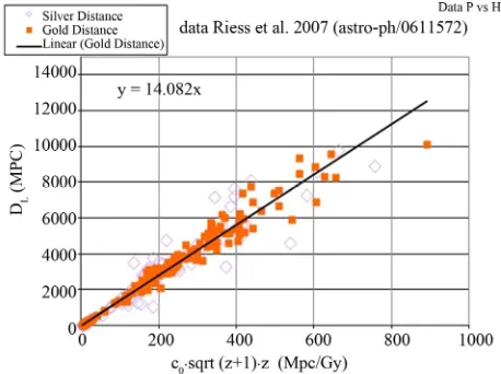
Figure 1 shows the measured distances provided by A.
Riess et al. [9] as a function of the red-shift z together with the calculated distance representing an expanding empty universe. Our universe is certainly not empty, but these distances are close to those calculated for a flat dark- energy model [8].
The fact that the speed of light is not necessarily a constant [1] and that a diminishing speed of light also puts the observations further away than a model in which the speed of light is constant, leads to a tempting modifi- cation of the Hubble Law by letting c(t)·z being the vari- able against which to plot the measured distances. The red shift is then a combination of the contribution by the expansion of the universe with scale a(t) and the contri- bution of the change in the speed of light c(t). It can be readily seen that with a conservation of the Planck con- stant ħ the red shift becomes:
0 0 0
obs c t λ
λ c a t
1 obs em em λ λ z
λ λ
(1)
The first ratio of the wavelengths is due to the expan- sion of the universe and the second part related to the change in the speed of light. In case c(t) = c0/a(t) one gets
a simple relation between a(t) and the red-shift z:
1 2
1
z
a t . And of course c(t) = c0·(z + 1)1/2. In
this way c·z = c0·(z + 1)1/2·z.
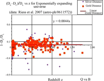
This relation is then given in Figure 2. The result
clearly points to the fact that the measured distance has the following relation to the red shift z:
1 z 1 1
0 0 L
D c t z (2)
This should be compared with the calculated one [8]:
Figure 1. Measured distances of the Supernovae from A. Riess et al. against the measured red shift z. Also shown is the calculated distance (solid black curve) against z for an empty expanding universe a(t) = t/t0 with t0 = 14.4 G year.
This calculated distance is very close to the one calculated for a flat dark energy model [8].
Figure 2. The measured distance DL versus the product c(t)·z in which c(t)= c0/a(t). c0 is the speed of light at present.
A remarkable good fit with the data is obtained with a char-acteristic time t0 of 14.082 G year.
0 1
0 0 now
1 ( )d 1 d
( ) ( ) ( ) t
t x
c t c t
D t z x
a t
a t a t
(3)
with x = t/t0.
The Equations (2) and (3) are very similar. This sug- gests that indeed a(t) = (z + 1)–1/2. From which together
with Equation (1) it can be seen that c(t) = c0·(z + 1)1/2 =
c0/a(t). Then it follows that (z + 1) scales as e(1–x).
Type of Expansion
Is the exponential expansion the only possible fit? In principle there are all kind of combinations of a(t) and c(t) possible that match Equations (2) and (3) and satisfy Equation (1).
Equating Equations (2) and (3) and eliminating c0·t0,
one gets:
1 1
2
1 d 1γ
x
z x z z
(4)If one stipulates that a(t) = (z + 1)ɣ, one can by varying
ɣ get a range of a(t) and c(t) pairs that satisfy Equation (1) and lead to the modified Hubble Law. For instance γ
= –1 represents the expanding universe with a constant speed of light. But all other possibilities lead to a varying speed of light over time. The nature of the red-shift limits the range of gamma to values of: –1 ≤ ɣ ≤ 0. A universe that would not expand at all is represented by ɣ = 0.
Differentiating Equation (4) as function of x yields:
1
32 d3
d 1
2 γ z z
x γ z
(5)
integration:
12
12 21
1 1 1
2 2 4
γ γ
γ
1 1
3 1
1
2 2
z z
x γ γ
γ γ
(6)
It should be noted that for γ ≈ –1/2 we have 1 – x≈ ln(z + 1) with a relative error of (γ + 1/2) ln(z + 1).
For ɣ = 0, this is the case of no expansion, we get:
2
(5 ) 12 6
x
(5 )
1 x
z (7)
Indeed x = 1 or t = t0 yields z = 0, x = 0 yields z = 0.43,
and x = –∞ leads to z + 1 = ∞.
This latter does agree with the observations that the red-shift always increases when looking back in time.
For γ = –1, this is the case of c(t) = c0, the speed of
light is a real constant, we get:
4 1
1
1 x
z
1 1
3 3 z 1
(8) For x = 1 one gets again z = 0, which is fine. This time however one gets z = ∞ at x = –1/3.
Equation (8) has one real root,
2 2
2
9 2
9 2
x
x
3
3
1 3 5 6
1
1 3 5 6
x x
z
x x
(9)
This is for small x + 1/3 close to:
2 1 1
1 3 x
z (10)
So one has a choice to make:
First of all one should realize that the modified Hubble Law required that c(t) = c0/a(t)and that therefore already
we have strong evidence for γ = –1/2.
Secondly, looking again at Equation (2) that was found from the measurements:
1 z 1 1
0 0 L
D c t z (2) And the definition of a measured distance (3):
1
0 0 1 d
( )x
c t
z x
a t
nowD (3)
The most obvious connection to make is to put:
1 1 ( )
z a t and
1(z1) dx(z 1) 1x
This then leads directly to: c(t) = c0/a(t)and z + 1 = e(1–x).
It is the most straightforward relation that we can ex- tract from Equations (2) and (3), but in principle it does not exclude other options discussed above.
The “obvious” connection leads to an expansion grow- ing exponentially in time: its scale factor is
a(t) = exp[(t/t0 – 1)/2]. The growth is slow with an
e-folding time of 28.2 G year.
Thirdly as shown in the discussion in Section 5, there is supporting evidence that the sizes of the galaxies scale as (z + 1)m, with –1 < m < 0. So that γ = –1/2.
It is interesting to note that for small z, (t close to t0)
one can expands a(t) and obtains a power scaling of a(t) ≈ (t/t0)1/2 . This would be the power scaling for a dense
universe with ρ > ρcr the latter being the critical density at
which the expansion of the universe is just not stopping [8]. So by letting the speed of light relax over time the universe can have density compared to the power scaling of a(t) = (t/t0) which fitted the data so good for the con-
stant speed of light model, but had zero density power scaling.
An exponential growth is structurally different from a power scaling. A power scaling has a beginning at t = 0, an exponential growth has no beginning (t = –∞ is the start of all) and it has no end. t0 is just an e-folding time
for (z + 1) and 2*t0 for a(t). But for sure the beginning
and the end of the universe are both well outside the measurements. It may well be that the beginning was linear and the end will be in a saturation state, in this case the exponential expansion can no longer be applied.
The quality of the fit of the exponential growth model to the Supernovae data is remarkable good. This is shown in Figure 3.
There is no systematic difference between the measured distances and the calculated one. In the case for the zero density power scaling [9] there is a positive difference. An accelerating dark-energy model was required to ex- plain this difference.
[image:3.595.54.292.81.542.2]An expansion accelerating in recent times is of course in agreement with an exponential growing expansion. But the latter came “naturally” out of the measured data itself.
[image:3.595.315.533.518.687.2]It is clear, that an exponentially growing expansion needs an “explanation” too in the form of dark energy that drives the growth.
3. The Expansion and Conservation Laws
It is necessary to check whether conservation laws re- main valid in these changing conditions. It should be noted that this section is valid for all combinations of a(t) and c(t), i.e. whether the speed of light is a real constant or not.
The first law to check is the energy conservation law for e.g. a planet of mass m orbiting a star with mass M at a distance r. The condition that the planet is in an orbit around the star gives the following condition:
2 M
v G
r
(11)
The energy is the kinetic plus potential energy, which equals:
2
1 2
kin pot pot
E E E mv
mv 2 2 2 3 3 2 2 mM G r v mc c (12)
With changing a(t) and c(t) energy is thus conserved if the ratio of v/c is conserved, since from relativity mc2 is
conserved. This implies too that the relativistic energies are conserved.
The law of angular impulse momentum is: 2
mv v r
ω
P m (13)
Since mv2 is conserved, angular impulse momentum
conservation would mean conservation of ω. Also it would follow then that r/c is conserved and this implies:
1 1γ( ) a t r
0
0 0
( ) ( )r ( 1) ( ) r t c t z a t r
c
(14)
It is clear that for –1 < γ < 0 Equation (14) leads to se- rious problems with the expansion condition that r(t) should be equal to r0·a(t).
Let us see how one can redefine the angular impulse momentum in such a way that the latter is conserved and the orbit can expand in the correct way. Put:
2 2 0 0 0 1 t v mc r c c ( ) ( ) v ( ) f P mvr f t mc a t r
c c
(15)
This gives: 0 ( ) 1 ( ) c t ( )
f t z
c a t
One
(16)
could state that: mc2
c a v r is conserved
and ular momentum (whi
ou e following orbita
P
define that is the ang ch it is in
r time). This leads to th l frequency:
0 0
0 ( )
( ) 1
( ) c t
ωt ω ω z
c a t
(17)
The same logic applies for the hydrog angular impulse momentum is:
en atom. The
0
e
c t
m v a t h
c a0 t
(18)
It then follows that the Bohr radius is:
0
0 2 0 0
e
a t h a t a t
m c α
c a t
(19)With th definition of the angular impulse
conservation implies that the scaling with the expansion sc
is momentum,
ale factor a(t) is maintained for both planet orbits and atoms.
The conservation of the electric charge has to be adapted to the expansion too.
The force balance in the hydrogen atom stipulates that:
2
e 2 2
0 0
mc α
ε a (20)
Therefore:
2 2 2 2 0 0 0 ( ) e emc α a a t t a t ε
(21)
And since ε0μ0=1/c2 one may assume th
ε0(t0)·c0/c(t). This leads to:
0
t ε
at ε0(t)=
0
2 2 2
0
1 c a t
e t e t c t e t0 z1 (22)
4. The Clocks and Expansion
he elec-Let us take as atomic clock the time it takes for t tron to go around the proton:
0
0 0
00 2π 0 0
τ t
a t c
τ t τ t a t
v t
(23)
1 c t z Also the orbit time for a planet around a sta
like that: Equation (17). r scales
How does the pendulum scales? One has to know how the gravitational constant scales with c and a(t). Energy conservation gives the following relation:
3
0 0
0 0
0 0 c0
In our case of c(t)·a(t) = c0 we get that G sca
the third power in c. But also in case of a consta of
c t c t a t m M r
G t G G
m M r c
(24)
les with nt speed light one has to take into account that G still scales then with a(t).
3 2
0 0 ( ) 0 0 ( )
( ) p
p
τ t a t c r
τ t 3
0 ( ) 0
g G c t M
2π 2π
1
z
(25)
We can conclude that the clock of the pendulum, the orbit period of planets and the orbit period of the e all change at the same rate in time: inversely proportional to
lectron
the red-shift z + 1. Note that also for a really constant speed of light the clocks would still scale like that too.
This dependence of the clocks has implications for the Lorentz equation and so on Relativity. It can be seen that Relativity is unaffected by the expansion of the universe.
The Lorentz equation is:
2 2 20
2 2 2 2 2 2 2 2 2 2
0 0 0 2 0
c c a t
x y z c τ a t x y z τ
c
(26) This just states that the Lorentz length too is multip ie by a(t). Since also all ratios of (v/c) are conserved, it fol-lows that Relativity remains unaltered.
the exponential nsion. It has been shown that the gal-is a function of the red-shift z [10]
ponential scaling law gives a very good match to servations. Exponential expansio rce. Dark Energy must be there. Power
7. Acknowledgements
ank the Mediterranean Insti-
REFERENCES
[1] P. Smeulders, eed of Light,” Su-
l d p
Also Quantum mechanics are unaffected. It can readily be seen that all energy levels of the Hydrogen atom are in units of mc2α2, which remain unchanged.
5. Discussion
There exists tempting supporting data for scaling of the expa
axy size (in kpc) . The
data in Figure 5 of reference [10] show that the size of galaxies scales as (1 + z)m, with m between 0 and –1. For
m = –0.5 the galaxies would scale as the scale factor of the expanding universe, namely as a(z) = (1 + z)–0.5. This
then supports the exponential expansion.
One can then conclude that starting from 50 Gyears ago (z = 5) the universe has been expanding exponen- tially.
6. Conclusion
The ex
the Supernovae ob quires a driving fo
n re-
scaling laws are not very suitable to describe the evolu- tion of the universe. Exponential expansion puts the Big Bang far back in time, but this is outside the measure- ments where we do not really know whether the expo- nential expansion remains valid. A modification of the
definition of the angular impulse momentum is required in order to get a consistent expansion of the universe even in case of a constant speed of light. The clocks in the universe scale inversely proportional to the red-shift z
+ 1.
The author would like to th
tute of Fundamental Physics i.e. Prof. A. Kavokin for his great interest in and support for this controversial topic. Also the author is much in debt to Dr. A. Riess for mak- ing the Supernovae data available in his publication.
“The Measure of the Sp
erlattices and Microstructures, Vol. 43, No. 5-6, 2008, pp. 651-654.doi:10.1016/j.spmi.2007.07.007
[2] J. K. Webb, et al., “Further Evidence for Cosmological Evolution of the Fine Structure Constant,” Physical Review Letters, Vol. 87, No. 9, 2001, Article ID 091301. doi:10.1103/PhysRevLett.87.091301
[3] A. Albrecht and J. Magueijo, “Time Varying Speed of Light as a Solution to Cosmological Puzzles,” Physical Review D, Vol. 59, No. 4, 1999, Article ID 043516. doi:10.1103/PhysRevD.59.043516
[4] J. D. Barrow, “Varying Constants,” Philosophical Trans-
, “A Simple Cosmological Model with De-
- actions of the Royal Society London, Vol. A363, 2005, pp. 2139-2153.
[5] J. C. Gimenez
creasing Light Speed,” 2003, arXiv:astro-ph/0310178. [6] J. W. Moffat, “Superluminary Universe: A Possible Solu
tion to the Initial Value Problem in Cosmology,” Interna- tional Journal of Physics D, Vol. 2, No. 3, 1993, pp. 351- 365.doi:10.1142/S0218271893000246
[7] E. Wright http://www [8] E. Wright
.astro.ucla.edu/~wright/cosmolog.html
.astro.ucla.edu/~wright/sne_cosmology.html http://www
[9] A. Riess, et al., “New Hubble Space Telescope Discover- ies of Type la Supernovae at z≥ 1: Narrowing Constraints on the Early Behavior of Dark Energy,” Astrophysical Journal, Vol. 659, No. 1, 2007, pp. 98-121.
doi:10.1086/510378