Operational Semantics Applied to Model Driven Engineering

(1)

T.J.L. Wolterink

Operational Semantics Applied

to Model Driven Engineering

Thesis

for the degree of

Master Of Science

(Computer Science, Track Software Engineering)

Supervisors

Dr. I.Kurtev

Dr.Ir. K.G. van den Berg

A. G¨oknil

(2)

(3)

Abstract

Model driven engineering (MDE) is an approach to software engineering and is used more and more in both research and practice. It provides a higher level of abstraction and supports domain specific languages (DSLs). There is much research done on the static aspects of MDE and most examples deal with static models. However DSLs are also used more and more to model the behaviour of a specific domain. These DSLs often lack clear and formal semantics.

Some approaches have been taken to define the semantics of modelling lan-guages. These approaches differ in their pragmatic and formal aspects. None of these approaches are built upon the existing formalism of Structural Oper-ational Semantics (SOS). SOS specifies the semantics of a language based on rules. These rules define a transition system in which the states are extended ASTs. This research adapts SOS in such a way that it can be applied on MDE models instead of ASTs. SOS seems to be a good candidate for specifying the se-mantics of modelling languages because it is based on the structure of programs which are well defined in a metamodel of a modelling language.

The main contribution of this thesis consists of a Semantic Language,SemLang, which is based on SOS. The Semantic Language is defined using an MDE ap-proach:SemLang is defined as a metamodel. It closely resembles SOS but has some differences that make it suitable for defining the semantics of a DSL based on metamodels. A SemLang model is a set of rules that defines a transition system where the states are extended models.SemLang has constructs to deal with lists and graph structures. The Semantic Language is formalized by altering the existing formalizations of SOS.

(4)

(5)

Acknowledgements

All the work done for this thesis could not be done without the help, encour-agement and support of numerous people. Different people supported me in different ways and this combination ensured a pleasant working environment. At first I want to thank my first supervisor, Ivan Kurtev, for his guidance before and during the project. Without his help I would have had difficulty discovering the interesting world of academic research. I also admire his calmness and informality, even when he had to supervise numerous other graduation students. I would also thank my other supervisors, Arda G¨oknil and Klaas van den Berg, for taking the time to read and review my thesis.

Secondly I want to thank my family; my brothers and especially my parents for supporting me throughout my years at the university. Even though it is difficult for them to understand the work done in my thesis I am sure they will try to read some parts of this thesis. Especially this paragraph.

Another important ingredient were my fellow students from room 5066 (for-merly 5070). The working atmosphere in that room was great on they provided help when needed. The discussions during lunch and during work were both entertaining and occasionally also informative.

At last I want to thank anybody that I forgot to thank. This includes the authors of the interesting papers I have read and of course anybody that showed interest in my work as a master student.

Tjerk Wolterink, August 2009, Enschede

”The sciences do not try to explain, they hardly even try to interpret, they mainly make models. By a model is meant a mathematical construct which,

with the addition of certain verbal interpretations, describes observed phenomena. The justification of such a mathematical construct is solely and

precisely that it is expected to work.”

(6)

(7)

List of Figures

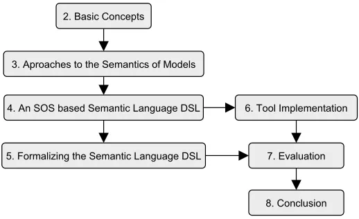
1.1 Dependencies between chapters . . . 5

2.1 Layers in MDE . . . 8

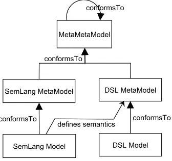
3.1 SemLang describes the semantics of a DSL . . . 21

3.2 Expression language metamodel . . . 22

3.3 Expression language sample model . . . 23

3.4 Semantic SOS rules for the expression language . . . 24

3.5 Execution states after applying the rules to the example model . 27 3.6 Simple imperative language metamodel . . . 28

3.7 Sample model as a graph . . . 29

3.8 SOS rules for binary expressions . . . 30

3.9 Rules for theSeq command . . . 31

3.10 Store definition and rules forAssignandVar . . . 32

3.11 First transition of the sample model . . . 33

3.12 Last transition of the sample model . . . 34

3.13 Functional language metamodel . . . 35

3.14 Sample model as a graph . . . 36

3.15 Evaluation of the definitions . . . 38

3.16 Evaluation of the SeqDef to an environment . . . 41

3.17 Reading a variable from the environment . . . 42

3.18 Concrete visual model of an Activity Diagram . . . 44

3.19 Activity Diagram language metamodel . . . 45

3.20 Object model of an Activity Diagram . . . 46

3.21 Example state transition for the example Activity Diagram . . . 50

3.22 Concrete visual model of an example Petri Net . . . 51

3.23 Petri Net language metamodel . . . 52

3.24 Example Petri Net model . . . 52

3.25 Petri Net example simulation . . . 53

3.26 Petri Net example model simulation . . . 56

5.1 Component Diagram of the Tool . . . 68

5.2 Class Diagram of the Semantic Engine . . . 69

5.3 Class Diagram of the UI . . . 71

5.4 The state graph view . . . 71

5.5 The transition stack view . . . 72

(12)

(13)

List of Abbreviations

ASM Abstract State Machine

AST Abstract Syntax Tree

BNF Backus–Naur Form

DSL Domain Specific Language

DSM Domain Specific Modelling

EMF Eclipse Modelling Foundation

EMOF Essential Meta Object Facility

GME Generic Modelling Environment

GMF Graphical Modelling Framework

GPL General Purpose Language

LTS Labelled Transition System

LTTS Labelled Terminal Transition System

MDA Model Driven Architecture

MDE Model Driven Engineering

MOF Meta Object Facility

MSOS Modular Structural Operational Semantics

OCL Object Contraint Language

OMG Object Management Group

QVT Query View Transformation

RCP Rich Client Platform

SemLang Semantic Language

SI Structural Induction

SOS Structural Operational Semantics

SWT Standard Widget Toolkit

TCS Textual Concrete Syntax

TSS Transition System Specification

UML Unified Modelling Language

(14)

(15)

1

Introduction

1.1 Background

Modelling is used to understand processes and systems in the real world. Dif-ferent formal and informal modelling languages have been introduced. This in-cludes petri nets, state charts and UML . Programming languages and human languages on the other hand can also be seen as modelling languages. These languages differ in their formality, ambiguity and application domain.

A new approach to software development is Model Driven Engineering (MDE) [Ken02]. MDE raises the level of abstraction by introducing metametamodels [B´04]. When defining a language without MDE one first specifies the concepts of the language (either mathematically or by using a syntax specification). Then one defines the semantics of the language in either an informal or formal way. With MDE one specifies a modelling language by creating a metamodel which describes the structures of the models. A textual or graphical concrete syn-tax can be created if needed (for example with TCS [JBK06]). However, there is no commonly established way of specifying the semantics of an executable modelling language. A simple approach is to use code generation, however, this approach is rather informal. Some research is done in the area of formal seman-tics for MDE; different authors apply different formal frameworks to solve this issue [SW08, Hec06, BH02, RRDV07, RV07, CCG+_{08, VPF}+_{06, CSAJ05].}

No research to adapt the Structural Operational Semantics (SOS) [Plo81] for-malism to MDE is done in the past. This forfor-malism seems a fruitful approach for MDE because the SOS formalism is built upon the structure of a modelling lan-guage. MDE has metamodels which clearly define the structure of a modelling language.

1.2 Problem Statement

Adapting SOS in order to make it useful in an MDE context is not straight forward. The first problem is the incompatibility between SOS and MDE; SOS is applied on trees while MDE models are graph structures. However, we think it is possible to apply SOS, with some changes, to MDE. This leads to the following research question:

Can SOS be adapted and applied successfully on MDE?

(16)

that need to be answered. The first sub-question is:

MDE models are graph structures but SOS is based on trees. Can SOS be adapted in order to make it suitable for using it with graph structures?

The main problem is the differences between the programs in SOS and MDE. In SOS the program is represented as a (extended) abstract syntax tree. In MDE, however, the program is represented as a model which is basically a more general graph structure. This difference is a problem that needs to be solved.

SOS is based on the abstract syntax description of languages, how can SOS be adapted to deal with metamodels?

The rules in SOS refer to the abstract syntax of a language in order to transform language structures to new language structures. In MDE metamodels have the same role as the abstract syntax description. This difference requires changes to SOS in order to apply it to MDE.

The semantic domain of SOS is a labelled transition system in which the states are trees. How can we change the semantic domain in order to make it suitable for models?

A semantic domain is a well known mathematical domain in which the semantics is expressed (for more details see section 2.5). The semantic domain of SOS is specified in different papers [Plo81, AFV01, Mos04]. The semantic domain of SOS is not suitable for defining the semantics of MDE modelling languages. It is of course difficult to test whether the main hypothesis is met in the end of the thesis. Therefore we limit the test to a set of DSLs which have different semantic properties. This includes imperative and functional languages but also graph like languages like petri nets and state charts. Another important result is to point out what the difficulties are when applying SOS to MDE.

1.3 Research Objectives

The research objectives are listed below. A description of each objective is given.

• Adapt SOS in order to make it suitable for MDE

The objective of this research is to adapt SOS in order to make it useful for MDE. This includes adapting the SOS formalism and specifying how it is related to the metamodel of the modelling language. The goal is to show that MDE and SOS are a good match by proof of concept.

• Introduce a new semantic language which is based on SOS

The main work in order to reach that objective is to develop a new se-mantic language based on SOS which can be used to define the sese-mantics of modelling languages. The focus should be on the pragmatic aspects.

• Provide a partial formalization of the new language

In order to provide some mathematical foundation for our work an impor-tant contribution is the partial formalization of the new language. This formalization can be built upon existing formalizations of SOS.

(17)

1.4. CONTRIBUTIONS

Another major objective is the development of a tool. The tool is needed in order to make the SOS based language useful. The tool should be able to load and simulate models given their semantics description. The addition of a graphical user interface is also desirable.

• Validate the research by applying the new language on some example DLSs The new language will be applied on several example DSLs in order to illustrate that the research goal is met. These example DSLs should cover different language types, like imperative and functional language. Part of this objective is to apply the new language on graph based languages like Activity Diagrams.

1.4 Contributions

Each objective resulted in at least one contribution. The contributions are listed below with a description accompanying each contribution.

• A newSemantic Language is introduced

This work introduces a Semantic Language which can be used to specify the dynamic semantics of modelling languages. The Semantic Language builds upon SOS and is therefore greatly influenced by the structure of SOS rules. However, the Semantic Language has features that make it suit-able for defining the semantics of modelling language defined using MDE concepts. The Semantic Language itself also follows the MDE principles; the language is defined as a DSL. It comes with a concrete syntax which makes it easy to define the semantics of a DSL.

• A partial formalization of theSemantic Language is given

The known semantics of SOS are adapted in order to provide the mathe-matical foundations for the Semantic Language. The main differences are in the semantic domain and in the rules. The states in the semantic do-main of the Semantic Language are basically extended graph structures. The rules consist of terms that refer to metamodel elements instead of AST elements.

• A solution to the problem of applying SOS with graphs

The main difference between the Semantic Language and plain SOS is that the Semantic Language is suitable for defining the semantics of graph based models. The main changes that were needed was the introduction of a breath-first-search based copy algorithm. This copy algorithm en-sures that nodes are not copied more that once, thus preventing infinite recursion.

• An implementation of a graphical tool calledSemantic Engine

(18)

• TheSemantic Language is applied to several example DSLs

Another contribution is the application of theSemantic Language to sev-eral example DSLs. This is done as a proof of concept. The DSLs cover a range of language types; functional and imperative languages but also graph based languages like Petri Nets and Activity Diagrams.

Different approaches for defining the semantics of DSLs already existed. How-ever, nobody tried adapting SOS in order to make it suitable for defining the semantics of DSLs. This thesis provides a first approach in combining SOS and MDE.

1.5 Outline

Chapter 2 introduces all basic concepts that are used in this thesis. It explains MDE and highlights some approaches in the MDE field. Secondly the use of do-main specific languages is explained. The redo-maining of the chapter focuses on the semantics of languages. The structural operational semantics (SOS) approach to semantics is explained in more depth.

Chapter 2.7 takes a look at the current approaches to specifying the semantics of models in an MDE context. Some current approaches are explained. These approaches must be explained to place this thesis into a proper context, it also provides some comparison material.

Chapter 3 introduces a DSL named SemLang which can be used to specify the semantics of other DSLs. The DSL is based on SOS but has some nice features that make it suitable in an MDE context. The chapter also provides some example DSLs on whichSemLang is applied.

Chapter 4 formalizes the DSL SemLang DSL. It builds upon existing formal-izations of SOS. The formalization provides a solid mathematical framework on which theSemLangDSL is built.

Part of this research was also the implementation of a tool which could simulate DSLs for which the semantics are defined using SemLang. The tool require-ments, architecture and evaluation can be found in chapter 5.

The evaluation of the work done in this thesis can be found in chapter 6. Our approach is compared to the existing approaches for defining semantics of mod-els. The conclusion of this paper is in the last chapter (chapter 7) in which the answers to the research questions can be found.

(19)

[image:19.595.142.401.332.490.2]

1.5. OUTLINE

(20)

(21)

2

Basic Concepts

2.1 Introduction

The main aim of the thesis is to introduce a framework which can be used to define the semantics of modelling languages in a formal way, therefore it is im-portant to investigate the basic concepts in this area. First the main concepts in the Model Driven Engineering (MDE)[Ken02] field are explained. The con-cepts of model and metamodel and the relations between them are explained. Subsequently some approaches to MDE are explained and their differences and similarities are discussed. In section 2.4 domain specific languages (DSLs) and their relation to the MDE field are covered. Novices in the MDE field may skip the first two sections.

In the end the current state of the art in the specification of the semantics of programming languages is explored. The knowledge in this area can be used to specify semantics for modelling languages. The next chapter (chapter 2.7) explores how the semantics of DSLs are currently specified.

2.2 Model Driven Engineering

Model Driven Engineering (MDE) provides a higher level of abstraction with respect to software engineering. Analogous to the principle everything is an object in object technology, MDE embraces the principle that everything is a model [B´04]. The notion of a model is a powerful unification concept in MDE, therefore it is important to know what a model is and how modelling languages are defined.

2.2.1

Models and Metamodels

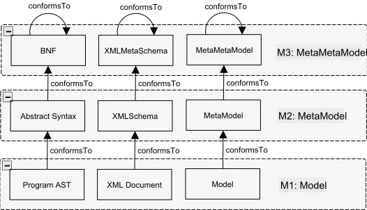
A model represents a system (part of the reality), and is expressed in a modelling language. In MDE the structure of the modelling language is given by another model, called its metamodel. This is a generalization of what is common in computer science (e.g., aJava program conforms to theJava grammar). Models and metamodels can be placed in layers, by MDE convention the real-ity is in layer M0, models that represent the reality are in layer M1 and the metamodels of those models are in layerM2.

(22)

Definition 1 (Model) A model (at M1) is an abstraction of a part of the reality for a specific purpose. A model is expressed in a modelling language.

Definition 2 (Modelling language) A modelling language is a well under-stood (not always formal) language which describes the concepts and their rela-tion of a part of reality.

[image:22.595.191.454.251.402.2]

Definition 3 (MetaModel) A metamodel (at M2) is a model of a modelling language.

Figure 2.1: Layers in MDE

Because a metamodel is a model it is expressed in a modelling language. The model of this modelling language is the metametamodel. This suggests infinite iteration, to limit the iteration of the conformsTo relation a metametamodel is said to conform to itself (e.g., the syntax of BNF is defined in itself). The metametamodelling layer is layer M3. The relations between the layers (M1, M2 and M3) can be seen in figure 2.1. This figure also shows that existing technologies like BNF and XMLSchema fit into this view.

Definition 4 (MetaMetaModel) A metametamodel (at M3) is a model of a modelling language which can be used to express metamodels. The model of the modelling language of the metametamodel is expressed by itself.

In MDE all metamodels ideally conform to the same metametamodel in theM3

(23)

2.2. MODEL DRIVEN ENGINEERING

2.2.2

Model Definition

Informally a model represents something in the real world and conforms to a MetaModel. The definition proposed by Thirioux et al [TCCG07] defines a model as follows.

Definition 5 (Model) Let C⊆Classes be a set of classes.

Let R ⊆ {hc1, r, c2i|c1, c2 ∈ C, r ∈ Ref erences} be a set of references among

classes such that:

∀c1∈C,∀r∈Ref erences,|{c2|hc1, r, c2i ∈R}| ≤1

We define a model hMV,MEi ∈M odel(C, R) as a multigraph over a finite set MV of typed objects and a finite set ME of labelled edges such that:

MV⊆ {ho, ci|o∈Objects, c∈C}

ME⊆ {hho1, c1i, r,ho2, c2ii|ho1, c1i,ho2, c2i ∈MV,hc1, r, c2i ∈R}

The definition shows that a model is basically a special kind of graph. The

conf ormsT orelation is not specified in the model definition. As we will see in

the next sub-section this is specified in the metamodel.

2.2.3

Metamodel Definition

Now we have a definition of a model we need a definition of a metamodel, again we follow the definition given by Thirioux et al [TCCG07]. A metamodel (also called a reference model in the paper of Thirioux) is defined as follows:

Definition 6 (MetaModel) A metamodel is a multigraph representing classes and references as well as semantic properties over instantiation of classes and references. It is represented as a pair composed of a multigraph (RV,RE)built over a finite set RV of classes, a finite set as a RE of labelled edges, with a property over models represented as a predicate function.

We define a reference model as a triple

h(RV,RE), conf ormsT oi ∈metaM odel such that:

MMV⊆Classes

MME⊆ {hc1, r, c2i|c1, c2∈MMV, r∈Ref erences}

conf ormsT o:M odel(MMV,MME)→Bool

The model is only valid if the following condition holds:

∀c1∈MMV,∀r∈Ref erences,|{c2|hc1, r, c2i ∈MME}| ≤1

where |A| is the cardinality of a set A. Informally this condition says that a specific reference from a class can only go to maximal one other class. The

conf ormsT o function specifies the semantic properties over instantiations of

the metamodel. This function is not further specified here. It simply evalu-ates to true when a model conforms to the metamodel. For an example of

the conf ormsT o relation with respect to EMOF we refer to Thirioux et al

(24)

Again it is important to understand that different MDE approaches use dif-ferent metametamodels and thus allow difdif-ferent metamodels and models. The metametamodel in the formal framework of Thirioux only contains classes and references. Most MDE approaches also allow attributes, class hierarchies and references with multiplicities.

2.3 MDE Approaches

MDE and its concepts where introduced by the Object Management Group (OMG) [Sol00]. However, other approaches where proposed as well. This section will discuss the main approaches to MDE and their differences and similarities. First the initial approach of the OMG is covered. Then the approach taken by the Microsoft Software Factory Tools (MS/DSL) [GSCK04] is discussed. In the end two similar approaches Ecore [ECO], from the Eclipse Modeling Foundation [EMF] , and KM3 [JB06] are covered.

2.3.1

Object Management Group

The Object Management Group (OMG) introduced the Model Driven Architec-ture (MDATM_{) . They started the development of a metametamodel called the}

Meta Object Facility (MOF) . This resulted in MOF 1.4 [OMG02] and MOF 2.0 [OMG03a]. This language is designed in such a way that it can be used as the metametamodel for UML [OMG]. However, this comes at a higher com-plexity. The OMG understood that a simpler metametamodel was needed and therefore defined Essential MOF (EMOF) as a subset of MOF. However, even EMOF is seen as rather big by the MDE research community. As we will see a simpler metamodel facilitates understanding and makes it a better candidate for formalization.

The semantics of MOF is informally described using text. Ambiguous interpre-tation of MOF can therefore not be prevented and may cause inconsistent tool implementations. The OMG approach is a rather ambitious approach and tries to cover all aspects of MDE, however, in our view it is better to start with a sim-ple pragmatical MDE approach and extend that if needed instead of enforcing a specific full blown approach.

2.3.2

MS Software Factory Tools

The Microsoft tools for Domain Specific Languages (MS/DSL) is a suite of tools to support for creating and using domain specific data for automating the soft-ware development process [GSCK04]. MS/DSL takes a pragmatic approach: the main focus is on tool support. The MS/DSL does not have a rigid specification, in fact there is no explicit metametamodel defined [BHJ+_05].

MS/DSL is a proprietary platform and its main aim is to generate code. It therefore comes accompanied with a code generator. However, the aim of MDE is much broader than merely code generation. For example there is no model transformation language in MS/DSL. The biggest disadvantage is that it is a closed platform and it does not have a large research community.

(25)

2.4. DOMAIN SPECIFIC LANGUAGES

This may be the reason that there is no explicit metamodel defined, this only makes the tool complex. This may be appealing for beginners in the MDE field; however, in the long run an explicit defined metamodel is really beneficial.

2.3.3

Eclipse Modelling Framework

The Eclipse Modelling Framework (EMF) project is a large modelling and code generation framework which can be used in an MDE context [EMF]. The project tries to align itself with the OMGs MDA approach. But an important aim of the project is to be useful in a practical sense. However, this does not undermine the theoretical aspects like we see with the MS Software Factory Tools. In fact the metamodel, named ECORE [ECO] is explicitly defined and is almost identical to EMOF.

EMF core advantage is that it has a rich user community and a lot of tools that can be used. There are code generation frameworks, model2text and model2model transformation engines, and rich editors available. This richness makes EMF the most commonly used MDE platform.

Another advantage is that there are some MDE approaches which are inte-grated with the EMF Framework. For example the Topcased Toolkit [VPF+_06]

is such an approach. Also the approach by B´ezivin which uses KM3 [JB06] as a metamodel has an implementation which allows models and metamodels to be transformed to models and metamodels that fit in the EMF framework. The KM3 approach also comes with a technique which can be used to define a concrete syntax for a modelling language. Jouault et al for example provides a way to define the concrete syntax for a specific metamodel using TCS [JBK06].

2.4 Domain Specific Languages

Most programming languages are general purpose languages (GPLs) , they are very rich and can be used in any problem domain. MDE can be used to specify the metamodel of a GPL, however, the real power of MDE is the decoupling of the model from the technical platform.

Programs often solve problems in some problem domain. The program, however, is some programming language that has (often) no relation with the problem domain. The translation of the requirements in the problem domain to the actual program is a difficult and intensive task.

Suppose that the problem domain could actually be modelled in some language specific to that domain. Such a language is called a Domain Specific Language (DSL). Such a language closes the gap between the problem and the imple-mentation. In fact DSLs have been successfully used in some problem domains [vDKV00].

(26)

A problem with DSLs is that they are difficult to design and implement and require higher initial costs [Hud98]. Here is where MDE comes into play: DSLs and MDE are a perfect match. The MDE approach makes the specification of a DSL much easier. Creating a DSL in the MDE context is often called Domain Specific Modelling (DSM) [KT08].

2.4.1

MetaModel

The syntax of textual languages is mostly defined using Bachus-Naur Form (BNF). This is also visualized in figure 2.1. The grammar of a language is the metamodel of the language and BNF itself is a metametamodel, in fact BNF can be described in itself.

When defining a model for a specific domain one uses domain concepts to express the model. These domain concepts must be captured in a metamodel for that domain. The metamodel for a DSL is analog to the grammar for a textual language. Therefore the structure of a DSL can is captured in a MetaModel and the concrete syntax can be captured using different tools within MDE (for example TCS [JBK06]).

2.4.2

Semantics

The metamodel for a specific domain only specifies the structure of the models. However, the semantic properties such as conditions over valid models and the behavioural semantics of a model (if any) are not specified. Semantics are as important as the structure of the language. Some argue that semantics are even more important than the structure [Hud98].

The semantics of a DSL can be specified in different ways. They can be specific informally using text or using model-to-code transformations. The semantics could also be specified in a formal way. More on the general aspects of semantics of languages can be found in section 2.5.

2.5 Semantics of Languages

Language definition deals with defining thestructureof the language. However, the meaning of those structures must also be defined. This meaning is defined by thesemantics of the language. The semantics of a language can be defined in different ways. This section explains what the semantics are and we take a look at different approaches for specifying semantics.

2.5.1

General Theory

Any language consists of a structure defined by some syntactic elements. De-pending on the type of the language these elements can be words, sentences, boxes, diagrams etc. However, these structures do not have a meaning with-out semantics. The semantics of a programming language essentially models the computational meaning of each program [Mos06]. In order to define the meaning a mapping is defined from the syntaxL of the language to a semantic domain

(27)

2.5. SEMANTICS OF LANGUAGES

So in order to define the semantics for a syntax definition on has to choose a semantics domain S and a mapping from the syntax to the semantic domain has to be made. This mapping defines the meaning of the syntactic elements. The next two subsections will dive into two dimensions of semantics; the for-mality of the semantics and the dimension of static and dynamic semantics.

Formal versus Informal Semantics

Programming language tutorials often explain the meaning the language by explaining them with text and code examples. Those tutorials explain the se-mantics in an informal manner which is easier for the reader.

However, the disadvantages of informal semantics are that they can be ambigu-ous and imprecise. The semantic domain and the mapping from syntax to the domain are not explicitly specified.

Formal semantics on the other hand have an explicit semantic domain, which is often a well known mathematical domain like natural numbers, graphs or labelled transition systems. The mapping to that domain is also explicitly given. Formal semantics are precise and computer readable. They can also be combined with rigorous mathematical techniques like validation, proofs, simulation etc.

Static and Dynamic Semantics

The semantics of a language can be divided into static and dynamic seman-tics. The static semantics deals with compile-time semantics like type checking and well-formedness constraints. These semantics are called static because these semantics can only be checked before running the program.

The dynamic semantics on the other hand models the runtime behaviour of the program. All observable behaviour of a running program is defined by the dynamic semantics.

2.5.2

Approaches

There are several approaches to specifying dynamic semantics. Some of these approaches are denotational semantics, axiomatic semantics, Abstract State Ma-chine semantics and action semantics [Mos06]. The axiomatic and denotational approaches are discussed briefly below. However, the focus of this thesis is on another approach named structural operational semantics (SOS). This approach is explained in a separate section.

Axiomatic Semantics

Axiomatic semantics [Hoa69] is based on mathematical logic. The semantics of a language are specified by making general assertions (or axioms) about syntactic structures in the language. These assertions are known asHoare triples written as {P}S{Q}. They consist of a precondition P, a syntactic structureS and a postconditionQ. An example assertion is for example:

{x=A}x:=x+ 1{x=A+ 1}

This assertion states that ifxequals A, then after execution of the statement

(28)

by a set of axioms which define the behaviour of all syntactic structures in the language.

Denotational Semantics

Denotational semantics was develop by Scott and Strachey at Oxford [SS71, Sch86]. In denotational semantics the meaning of a language is defined by a set of functions, or denotations. Each denotation of a construct has a set of arguments that represent the information before its execution and a result that represents the information available after its execution.

Denotational semantics has been used to define the semantics of functional pro-gramming languages. However, attempts to give semantics to larger program-ming languages have been less successful [Mos06].

2.6 Structural Operational Semantics

Structural Operational Semantics (SOS) was first introduced by Plotkin in 1981 [Plo81] and has been researched further by other researchers [Hen90], notably Mosses [Mos02, Mos04]. SOS has been used to define the semantics of process algebras [Mil90] and programming languages [IPW01]. SOS is a compositional: the semantics of a phrase is specified by the semantics of the subphrases. Com-positional rules are used to specify the semantics of a specific language structure.

2.6.1

Semantic Domain

The semantic domain of SOS is a labelled transition system (LTS) (see definition 7), which is a well-studied mathematical object.

Definition 7 (Labelled Transition System) A LTS is a triple (Q, A,→)

with Q as set of states, a set A of labels α, a relation →⊆ Q×A×Q of labelled transitions ((s, α, s‘)is written as s−→α s‘).

The mapping from the syntactic domain of a language to the semantic domain is done by defining a SOS specification. A SOS specification consists of a definition of the states and a set of rules which define the transition relation in the LTS. The states are often sentences of the language with some extensions.

2.6.2

Rules

SOS rules are based on the abstract syntax of a language. A rule consist of assertion of transitions t−→α t′ _{where the terms}_t_,_t′ _{are syntactic constructs of}

the language which contain meta-variables and αis the label of the assertion. A rule is written as follows:

c1,· · ·, cn

c (2.1)

Wherec, c1,· · · , cn are transition assertions in whichc1,· · ·, cn are the

(29)

2.6. STRUCTURAL OPERATIONAL SEMANTICS

2.6.3

Example

In order to understand the rules the abstract syntax and SOS rules for a simple expression language will be given. Consider the abstract syntax of a simple expression language as defined below:

hExpi →n| hBinaryExpi hBinaryExpi → hExpi hExpi

This is the abstract syntax for a simple language in which the sentences are numbers nor binary expressions. In order to keep the language simple we did not add any operators for the binary expressions. In this case a binary expression is simply an expression which has two sub expressions. A simple sentence of this language is visualised as an abstract syntax tree below:

Exp

BinaryExp

Number

5

Number

3

n

2

This simple language will be used to illustrate how SOS is used to define the semantics of a language. In order to specify the semantics for this simple lan-guage we must know what the intended behaviour of the lanlan-guage is. In this case we simply evaluate a binary expression to the sum of its sub-expressions. Therefore a sentence in this language will always evaluate to a number. The SOS rules that specify this behaviour can be seen below. The rules con-tain meta-variables x, ei and ni. The meta-variable x matches any syntactic

construct, the meta-variableei only matches binary expressions and the

meta-variableni only matches numbers.

e1→e′1

BinaryExp(e1, x)→BinaryExp(e′1, x)

(2.2)

Rule 2.2 consist of a conditione1→e′1 and a conclusion. The condition can be

interpreted as:there is a rule which transforms the syntactic construct bound to

e1to a new syntactic constructe′1. The conclusion of the rule simply states that

in order to evaluate a binary expression one must first evaluate the first child expression.

e2→e′2

BinaryExp(n1, e2)→BinaryExp(n1, e′2)

(2.3)

Rule 2.3 matches binary expressions in which the first child is already evaluated to a number (which is bound to meta-variablen1). The rule states that if the

second child, bound toe2, of a binary expression evaluates toe′2then the binary

expression will evaluate to a new binary expression in which e2 is substituted

bye′ 2.

n=n1+n2

BinaryExp(n1, n2)→n

(30)

The last rule, rule 2.4, evaluates a binary expression, with two numbersn1 and

n2 as children, to the sum of those numbers. The conditionn=n1+n2 is not

a transition condition but simply an assertion.

Note that the three rules presented here do not strictly follow a specific rule format. They are just presented here to give you an intuitive understanding of SOS. To get a more in depth understanding of SOS it is recommended to read some papers on SOS, for example the paper by Plotkin [Plo81].

2.6.4

Transition System Specification

The semantic domain of SOS is a LTS. The states of the LTS are extended syntactic constructs of the language. The transitions between the states are specified inductively using the rules. Thus in fact an SOS specification specifies a LTS and is therefore called a Transition System Specification (TSS) . For a formal definition of TSSs and SOS we refer to papers by Mousavi et al [MRG07]. In this introduction we will just explain how a transition in the LTS can be proved by a set of rules. Such a proof is called a proof-tree. We define a proof tree in a similar way as Peter Mosses does in his paper about Modular Structural Operational Semantics (MSOS) [Mos04].

Definition 8 (Transition Proof Tree) Given a set of rules, a triple(s, α, s‘)

is in the transition relation of the LTS if and only if afinite upwardly branch-ing tree (the proof tree) can be formed that follows satisfies the following conditions:

1. All nodes are labelled by elements ofQ×A×Q

2. the root nodes is labelled by(s, α, s‘)

3. for each node withn child nodes there is a rule c1,···,cn

c and an

interpre-tation of the meta-variables such that

• the label of the node is the interpretation ofc

• the labels of the child nodes are the interpretations of c1,· · ·, cn.

The paper of Plotkin [Plo81] gives some examples of how to create a proof tree. Chapter 3 of this thesis shows how to create a proof tree using the proposed

Semantic Language.

2.6.5

SOS Styles

Different authors use SOS in different application domains. However, this re-sulted in a range of SOS styles [MRG07]. In order to choose an appropriate rule format for the Semantic Language we must be aware of the current rule styles and their features.

One important distinction in SOS approaches is thesmall-stepapproach and the

big-step approach. In thesmall-step SOS each transition generally corresponds to an indivisible item of information processing. In big-step SOS (also called

Natural Semantics) a computation is a single transition that leads directly to a terminal configuration. For intuitive examples of bothbig-step andsmall-step

(31)

2.7. APPROACHES TO DEFINING THE SEMANTICS OF MODELLING LANGUAGES

In general the small-step style will require a greater number of rules than the same specification in big-step style. However, the small-step style rules tend to be simpler. Another advantage of the small-step style is that it facilitates the description of interleaving. Thebig-step style can become ambiguous with respect to interleaving because thebig-step style rules do not enforce a specific order.

Other important characteristics of different SOS styles are described in the paper by Mousavi et al [MRG07]. We will not list the SOS formats described in that paper (there are more than 17 formats). However, an important conclusion of the paper is that negative and infinite conditions are a complicating factor in SOS frameworks.

2.7 Approaches to defining the Semantics of

Mod-elling Languages

2.7.1

Introduction

The problem of defining the semantics of a modelling language is not new. Some considerable amount of research has already been done, this has led to a number of approaches for defining the semantics. This chapter discusses existing approaches and gives advantages and disadvantages of the different approaches. This chapter also provides an initial bridge between the MDE and the semantics of languages in general as explained in the Basic Concepts chapter. It also provides comparison material which is used in the evaluation of this thesis. The sections in this chapter will cover the existing approaches like model trans-formations, graph transtrans-formations, Maude, the Topcased Toolkit and semantic anchoring.

2.7.2

Model Transformations

A powerful technique in MDE is model transformations. The unifying concept in MDE ”Everything is a model” makes the description of model to model trans-formation a relatively easy process. One standard for model transtrans-formations is the QVT (Query/View/Transformation) [OMG08] language as proposed by the Object Management Group (OMG).

The model transformation technique is used by Sadelik and Wachsmuth [SW08] to specify the semantics of a modelling language. The approach uses a LTS as the semantic domain. The states (orconfigurations as called by Sadelik and Wachsmuth) are models that conform to theconfiguration metamodel. The tran-sitions in the LTS are specified by a QVT model-to-model transformation. An

initialisation transformation is also needed which transforms a model to the first initial state model.

The authors built an Eclipse plugin, namedEProvide, which relies existing tech-nologies like EMF [EMF], MOF [OMG02, OMG03a] and QVT.EProvide uses Graphical Modelling Framework [GMF] to visualize the intermediate states dur-ing simulation.

(32)

[OMG03b] to define the model-to-model transformation. The transformation is defined graphically which is an advantage according to the authors.

2.7.3

Graph Transformations

Graph transformations [Hec06, BH02]is similar to model transformations how-ever as the name suggests, it is based on graphs as first class entities. To use graph transformations in MDE one has to create atype-graphfrom the language metamodel. The semantic domain is also a LTS. The states in the LTS are graph with a structure-preserving mapping to the type graph. Therefore it is required to transform a model to a graph before using it with graph transformations. Similar to SOS, the semantics are specified using a set of rules. A rule basically consists of two graphsLandR. The first graphLrepresents the pre-conditions of the rule and the second graphRrepresents the post-conditions. Intuitively a rule matches some part of the state graph and deletes/adds edges and nodes in order to create a new state. A rule is often created with a visual graph editor which makes graph transformations inherently a visual approach to specifying semantics.

Because graph transformations are built upon graph theory it has a sound math-ematical base. The semantic domain, the type-graphs and the rules are all for-mally defined. However a disadvantage of graph transformations is that the rules tend to become big; there is always a one-to-one relation between a transition in the LTS and a rule.

2.7.4

MDE with Maude

Maude is a high level language and an efficient rewriting engine that integrates functional programming with rewriting logic and provides metalanguage capa-bilities. Because of the facilities and capabilities of Maude it is used as a notation and semantic framework for specifying semantics of models and metamodels by Rivera et al [RRDV07, RV07, RGdLV08].

In the approach with Maude they first transform a language metamodel to Maude objects. Models are also represented as Maude objects and the Maude type system is used to check the validity of a model given its metamodel. The mapping from the MDE domain to the Maude domain is needed in order to use the Maude rewrite system for specifying the semantics of the modelling language.

The behavioural semantics of a modelling language are specified in Maude in terms of rewrite rules. These rules are added to the specification of the meta-model and meta-model in Maude objects. The Maude rewrite rules are similar to the graph transformation rules but are based onrewrite-theory and are specified in a textual form.

The Maude team is currently working on more model operations and on better tool integration with tools like MOF, EMF and KM3 [OMG03a, EMF, JB06].

2.7.5

Simulation in the Topcased Toolkit

The Topcased Toolkit [CCG+_{08, VPF}+_{06] is built upon the EMF Framework}

(33)

2.8. CONCLUSION

In order to use Topcased for a given modelling language one has to create dif-ferent metamodels. The initial metamodel of the language is called the static metamodel within Topcased. In order to define the semantics one has to create anevent metamodel which models all possible events that occur during simula-tion. Adynamic metamodelwhich relies on thestatic metamodel is used during the simulation. Thisdynamic metamodel may be used to specify some runtime elements that are needed to execute the model. Finally a trace metamodel is needed. This metamodel is used to define simulation scenarios as a sequence of events.

The actual semantics are defined in a pragmatic way: a component must be defined which implements the execution semantics using the programming lan-guage Java. EMF is used as a framework to update the structure of the model [EMF].

2.7.6

Semantic Anchoring

Semantic Anchoring [CSAJ05] uses yet another different approach. Essentially semantic anchoring uses model-to-model transformations to transform a model, for which the metamodel has no clear semantics, to a model for which the semantics is formally defined. One first defines a minimal modelling language

Lifor a well known mathematical domain (for example Abstract Sate Machines

(ASM) ). The abstract syntax and semantics of this language must be precisely specified. In order to specify the semantics of a modelling languageLa mapping (or model transformation) much be made between the abstract syntax of Lto the abstract syntax of Li. This mapping MA is called the semantic anchoring

ofLtoLi.

The GME [GME] tool suite is used for defining the abstract syntax of DSLs. The GReAT [GRe] tool suite is used to define the semantic anchoring. In the paper [CSAJ05] abstract state machines are used for the minimal modelling language

Li, the semantics ofLi is specified as an AsmL specification.

An advantage of Semantic Anchoring is that one does not have to define the formal semantics of a DSLL, only a model transformation from that DSL to a DSL with formal semantics Li is needed. However, this is not always possible

because a DSL may have semantic properties that are very different from Li.

Another disadvantage is that during simulation one does not simulate the model that conforms toLbut a model that conforms toLi. This may complicate things

and tracing between the two models must be needed in order to find bugs.

2.8 Conclusion

This chapter introduced all the basic concepts and contains references to re-lated work. The MDE approach is explained and definitions for models and metamodels are given. Different MDE approaches are covered and compared. We also showed the use of Domain Specific Languages and their relation with MDE.

(34)

more rules, the rules in the small-step approach are generally small and the rules only refer to directly accessible elements.

This chapter also covered different approaches for defining the semantics of modelling languages. In all approaches there is a mapping from the modelling language to a semantic domain. However, this mapping is done in different ways. Most approaches specialized LTS as the semantic domain, however the transition relation in the LTS is specified in different manners.

(35)

3

An SOS based Semantic Language DSL

3.1 Introduction

Semantics of models can be expressed in different ways. This chapter takes a MDE approach to specifying dynamic semantics. We will create a DSL, named

SemLang (an abbreviation forSemantic Language), which can be used to

de-scribe the semantic of other DSLs.SemLangwill be built upon existing knowl-edge about SOS and MSOS.

This chapter explainsSemLang informally with the aid of examples. A formal definition will be given in chapter 4. The examples start with a definition of a DSL, sequentially the semantics of the DSL is defined using SemLang. Each section adds more complexity toSemLang. After this chapter the reader should have a complete but informal understanding of SemLang and the differences between the well known SOS (Plotkin style) andSemLang.

[image:35.595.189.357.508.666.2]

In this chapter we will use the term DSL for the language for which the semantics is described. The difference between theSemLang and the DSL for which the semantics is described is crucial. This is visualized in figure 3.1.

Figure 3.1: SemLang describes the semantics of a DSL

(36)

correct-ness. This chapter, however, does not deal with formalization and is meant to be relatively easy reading. This is done to facilitate the understanding of the formalization in the next chapter.

Note that the metamodels and models defined in this chapter are built using the Eclipse Modelling Framework [EMF]. EMF is chosen because it has explicitly defined metametamodels and the tool support is well developed. For further reasons see section 2.3.3. Therefore the metamodels in this chapter conform to the ECORE metametamodel [ECO]. BecauseSemLang is a DSL itself it must also have a metamodel. The metamodel is too big to include here, but it is included in appendix A on the disc.

3.2 SOS for Expressions

In this section we will define a simple expression language by giving its meta-model. A small sample model is also given. The semantics is explained both informally as well as formally using SemLang. In the end of this section the sample model will be simulated by applying the semantics.

3.2.1

Metamodel

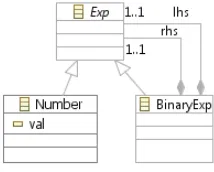
[image:36.595.267.374.476.562.2]

First the semantics of a simple expression language will be defined. The expres-sion language only consists of the conceptsExpression,Numberand Binary-Expression. The metamodel is given in figure 3.2. Models of the metamodels are either numbers or expressions. Also note that the models are always trees, this is because thelhs andrhs relations of a binary expression are containment relations (as specified by metametamodel ECORE [ECO]).

Figure 3.2: Expression language metamodel

An example model that conforms to the expression language metamodel is given in figure 3.3. The meaning of the nodes is explained in the list below:

• Black nodes represent objects, the label of the node is the name of the class that it conforms to.

– The outgoing edges of an object node are either references or at-tributes

– Black outgoing edges are containment references

– Green outgoing edges are attributes

(37)

3.2. SOS FOR EXPRESSIONS

• Green nodes represent attribute values

Figure 3.3: Expression language sample model

The example model is needed to show how the semantics is applied to a spe-cific model. Before the model can be executed the semantics of the expression language must be defined.

3.2.2

Semantics

The semantics of the expression language is very simple: a binary expression evaluates to the sum of its operands. The result of a full computation is therefore the sum of all the numbers in the model. This description is of course incomplete and informal.

The semantics must be described formally using a flavour of SOS suited for DSLs. As explained in section 2.6 an SOS specification consists of a number of rules. These rules specify the transition relation between states when executing a model. A transition is only valid if a tree of rules can be constructed which explain the transition (for full details see [Mos04]).

Because of the simplicity of the expression language we can create SOS rules with minimal modification to the format of the rules. Plotkin style SOS [Plo81] uses the syntax of the language in the rules. As explained in section 2.2.1 a metamodel plays the same role in a DSL as the syntax does in a textual language. Therefore we change the format of the rules in such a way that we refer to the metamodel instead of the syntax. The rules for the expression language are given below. The first equation is not a rule, it declares which states are end states (computed states). This is needed for every SOS specification to indicate when an end state is reached. The end state specification is rather simple: it declares that objects that conform to theNumberclass are end states.

(38)

Computes={Number} (3.1)

L→NL

BinaryExp(lhs= L,rhs= R)→BinaryExp(lhs= NL,rhs= R) (3.2)

R→NR

BinaryExp(lhs=L,rhs= R)→BinaryExp(lhs=L,rhs= NR) (3.3)

BinaryExp(lhs=L,rhs=R)→Number(val= (L.val+R.val)) (3.4)

Figure 3.4: Semantic SOS rules for the expression language

which matches objects that conform to the BinaryExpclass, the variables L and R are bound to the value oflhs andrhs respectively.

There is one subtle difference between the patterns in the rules; the variableL

is italic in the second rule, and both L and R are italic in the last rule. Italic variables are called computed variables. Computed variables can only bind to a computed value, as defined by the equation Computes= {Number}. If a computed variable cannot be bound then the rule does not match. This is also a subtle difference with respect to the Plotkin rule format. Plotkin uses different symbols for computed values (for examplemandn for numbers). Note that non italic variables can also match computed values: italic variables match a subset of what non-italic variables match.

Rule 3.2 and 3.3 come with conditions like L → NL. The variable at the left side of the arrow (L) in the condition must be bound to an object in the pattern of the rule. The condition holds if there is a rule x that matches the object to which L is bound to. If there is a rule found then NL is bound to the result of the application of rulex. If such a rule cannot be found then the condition does not hold. If a condition does not hold then the rule itself does not match. The variable at the right side of the arrow (NL) can be used in theresult of the rule. Theresult of a rule looks similar to the pattern. However, it is more complex and has a different purpose: it constructs new objects. For example the rule 3.2 has the result BinaryExp(lhs= NL,rhs= R). This constructs a new object that conforms to theExpression class and setslhs to acopyof the object to which the variable NL is bound to. Therhs reference is bound to thecopy of the object to which the variable L is bound to.

The copy algorithm can be kept simple in this case. This is because the meta-model of the expression language does not have cross-references; the meta-model will always be a tree. Therefore the copy algorithm only has to deal with trees. The copy algorithm simply copies the current object and its complete tree. The last DSL for which we describe the semantics (in section 3.5) does contain cross references. The complete copy algorithm is explained there.

The result in rule 3.4Number(val= (L.val+R.val)) constructs aNumber

(39)

3.2. SOS FOR EXPRESSIONS

Plotkin could not embed these expressions directly in the rules because they could interfere with the syntax of the language for which the semantics were described. Because theSemLangrule format does not refer to the syntax of the DSL we can simply embed these calculations in the rules.

3.2.3

Example Simulation

The semantics of the expression language is specified: the end state is defined and the rules are given and their format is explained (informally). The sample model in figure 3.3 can now be executed. The semantics of the expression language is modelled by a transition system. A transition system consists of states and transitions. Execution in the sense of SOS is a path in a transition system. The path consists of states and transitions from state to state. The last state is a valid end state. Each transition is proved by a tree of rules.

ExecutionP ath=State1→State2→ · · · →Staten−1→Staten=EndState

The transitions can be labelled, but for now they will not be labelled. The transitions are specified by the rules. However, we must clearly define the states of the transition system. The result part of every rule creates a new object that conforms to the metamodel. There are no elements created that are not defined by the metamodel. Therefore in this stage the states can be defined as models that conform to the metamodel of the DSL (the expression language).

When executing the sample model the first state is identical to the sample model itself. This state is not an end state because the root object does not conform to aNumber. Therefore all rules that match will be applied to create the new state. Only rule 3.3 matches.

Rule 3.2 does not match because the transition condition L→NL does not hold: the L was bound to value of thelhs, which is aNumberobject. The transition condition did not hold because there was no rule found which matches the L

Numberobject.

Rule 3.3 does match because the computed variableL was successfully bound to thelhs object. Variable R was bound to therhs object, which conforms to a

BinaryExp. The transition condition R→NR holds because a rule could be found which matches the R object: This is rule 3.2.

At this stage the variable L will be bound thelhswhich is a BinaryExp. The variable R is bound to therhs which is aNumber(where attributeval equals 2). Note that rule 3.3 does not match because thelhswas not a computed value. The transition condition L→NL of also holds because the last rule 3.4 which transforms a binary expression to a number can be applied.

The complete proof for the transition can be given by expanding the transition conditions. The first rule that is matched is rule 3.3:

R1→NR1

BinaryExp(lhs=L1,rhs= R₁)→BinaryExp(lhs=L1,rhs= NR₁)

(40)

L2→NL2

R1=BinaryExp(lhs= L2,rhs= R2)→NR1=BinaryExp(lhs= NL2,rhs= R2) BinaryExp(lhs=L1,rhs= R1)→BinaryExp(lhs=L1,rhs= NR1)

The transition condition L2→NL2 can be expanded by applying rule 3.4:

L2=BinaryExp(lhs=L3,rhs=R3)→NL2=Number(val= (L3.val+R3.val))

R1=BinaryExp(lhs= L2,rhs= R2)→NR1=BinaryExp(lhs= NL2,rhs= R2) BinaryExp(lhs=L1,rhs= R1)→BinaryExp(lhs=L1,rhs= NR1)

This gives a complete proof for a transition condition to a new state. The proof can now be used to construct the new state. This is done by substituting vari-ables with the constructed objects in each rule:

L2=BinaryExp(lhs=L3,rhs=R3)→NL₂=Number(val= (L3.val+R3.val))

R1=BinaryExp(lhs= L2,rhs= R2)→NR1=BinaryExp(lhs= NL2,rhs= R2) BinaryExp(lhs=L1,rhs= R₁)→BinaryExp(lhs=L1,rhs= NR₁)

NL2=Number(val= (1 + 5))

R1=BinaryExp(lhs= L2,rhs= R2)→NR1=BinaryExp(lhs= NL2,rhs= R2) BinaryExp(lhs=L1,rhs= R₁)→BinaryExp(lhs=L1,rhs= NR₁)

NR1=BinaryExp(lhs=Number(val= 6),rhs= R2) BinaryExp(lhs=L1,rhs= R1)→BinaryExp(lhs=L1,rhs= NR1)

Therefore the new state can be constructed using the following constructor. Note that the free variables in this constructor are bounded to objects.

BinaryExp(lhs=L1,rhs=BinaryExp(lhs=Number(val= 6),rhs= R2))

For each state we can find all possible transition by finding proofs for the tran-sitions. If the DSL is deterministic the only one proof can be found. The new state can be constructed by using the proof for the transition.

(41)

3.3. INTRODUCING THE STORE BinaryExp Number lhs BinaryExp rhs BinaryExp Integer:1 Number val Integer:2 Number val Integer:7 val Number Integer:5 val BinaryExp lhs rhs rhs lhs Number lhs BinaryExp rhs BinaryExp Integer:6 Number val Integer:7 val Integer:2 Number val lhs rhs Number rhs Number lhs Number Integer:8 val Integer:7 val Integer:15 val

Figure 3.5: Execution states after applying the rules to the example model

3.3 Introducing the Store

This section introduces a simple imperative language. First the language will be explained by defining the metamodel and giving a small sample model. Then the semantics will be defined using SemLang. This requires that SemLang must be extended to deal with a store. In the end the semantics will be applied to the sample model.

3.3.1

MetaModel

The imperative language consists of binary expressions as explained in the previ-ous section. However, a binary expression also has an operator. In this language we only have aPlusand aMinusoperator.

The simple imperative language given in this section also allows occurrences of variables; a value can be assigned to them and their value can be retrieved. Therefore a new expression is added: theVarexpression.Varevaluates to the value of the variable that it is referring to.

The main difference is that the imperative language given here allows commands to be executed sequentially. A command is either aSeqcommand or anAssign

command. A complete metamodel is given in figure 3.6. The given language is almost identical to the language given by Plotkin in chapter two of his paper [Plo81]. The main difference is again that our language is a DSL defined as a metamodel.

(42)

Figure 3.6: Simple imperative language metamodel

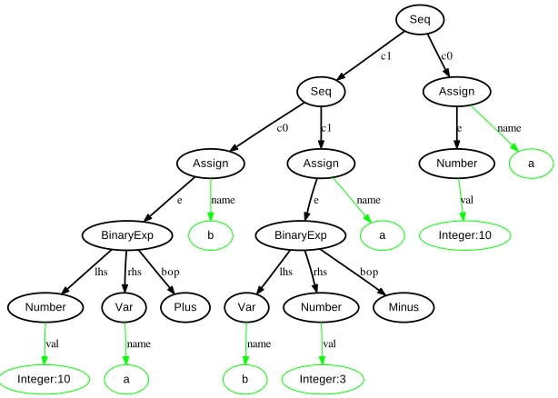
Representing an example model of this language as a graph tends to become large. Therefore the example model will be given in textual form to accommo-date easier understanding. However, this requires that we give a syntax definition for the metamodel. This is done by using the Textual Concrete Syntax (TCS) technology as defined by Jouault, B´ezivin and Kurtev [JBK06].

Listing 3.1: TCS for the simple imperative DSL

1 template Exp main abstract; 2 template Number : v a l ; 3 template Var : name ;

4 template BinaryOp abstract; 5 template P l u s : ”+”;

6 template Minus : ”−”;

7 template BinaryExp : ” ( ” l h s bop r h s ” ) ”; 8 template Com main abstract;

9 template A s s i g n : name ”:=” e ; 10 template Seq : ” ( ” c0 ” ; ” c1 ” ) ” ;

This TCS specification can be used to represent a model in textual form. An example model is given below.

Listing 3.2: Textual sample model

1 ( a : = 1 0 ;

2 ( b:=(10+ a ) ;

3 a :=( b−3)

4 )

5 )

(43)

[image:43.595.120.427.134.353.2]

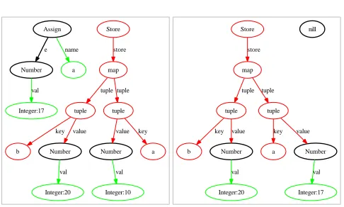
3.3. INTRODUCING THE STORE Seq Seq c1 Assign c0 Integer:10 Var b name BinaryExp Number lhs Var rhs Plus bop Assign e b name BinaryExp lhs Number rhs Minus bop Integer:3 val Assign e a name Number val Integer:10 val a name c0 c1 a e name

Figure 3.7: Sample model as a graph

3.3.2

Semantics

The semantics of the simple imperative language is first explained informally. Expressions are evaluated analogous to the semantics of the expression language (as explained in the previous section). The only difference is that the calculation that must be performed is specified by the operator, eitherMinfor subtraction or Plusfor addition. The Var expression is evaluated by getting the value of the referring variable from the store (internal memory).

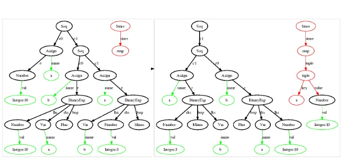
ASeqis executed by first executingc0 and then executingc1. AnAssignment is executed by first executing the expression and then by updating the store by binding the calculated value to the name of the variable. Executing a command does not yield a result.

The informal description of the imperative language includes the need of memory in which variables can be created, read, updated (and deleted). Therefore we add the concept of store, which is an abstraction of memory, to ourSemLang

just like Plotkin did in chapter 2 of his paper [Plo81]. In the approach of Plotkin a store is a function from names to values. To keep our approach flexible we define a store as a function from (ECORE) objects to other objects: Store :

Object→Object.

Each object has its own identity. When an object gets created it is assigned an identity. If it is copied then the copy gets a new identity. An object equals another object if it has the same identity. However, primitive objects like strings and integers have a different identity; they have the same identity if their values are equal.

(44)

the labels. However, internally the store will be added to a state. This is more readable and avoids using the use of category theory that MSOS requires.

The SemLang rules for the imperative language are explained step by step.

First some simple rules are explained and then more complex rules that deal with the store are explained. The new constructs that are added to SemLang

will also be explained.

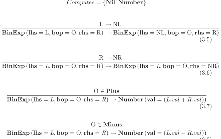
The rules for BinaryExp are almost identical to the rules for the expression language. These are presented in figure 3.8. An additional construct in the rules is a type-check condition. For example the condition O ∈ Plus holds if the object bounded to O conforms to thePlusclass in the metamodel.

Computes={Nil,Number}

L→NL

BinExp(lhs= L,bop= O,rhs= R)→BinExp(lhs= NL,bop= O,rhs= R) (3.5)

R→NR

BinExp(lhs=L,bop= O,rhs= R)→BinExp(lhs=L,bop= O,rhs= NR) (3.6)

O∈Plus

BinExp(lhs=L,bop= O,rhs=R)→Number(val= (L.val+R.val)) (3.7)

O∈Minus

[image:44.595.149.509.284.510.2]

BinExp(lhs=L,bop= O,rhs=R)→Number(val= (L.val−R.val)) (3.8)

Figure 3.8: SOS rules for binary expressions

Notice that the set of computed values{Nil,Number}includesNil.Nilrefers to a pseudo-object that represents no value, or no object.Computes={Nil,Number}

defines therefore that theNilpseudo-object or aNumberobject is a valid end state.

The introduction ofNilmeans that the states are not pure models that conform to the DSL metamodel. A state now must conform to a different metamodel that is an extension of the DSL metamodel. The only extension is that any reference may also point to aNilobject.

Next the rules that deal with theVarexpression and the commands (Seq and

(45)

3.3. INTRODUCING THE STORE

C0→NC

Seq(c0= C0,c1= C1)→Seq(c0= NC,c1= C1) (3.9)

Seq(c0=C0,c1= C1)→C1 (3.10)

Figure 3.9: Rules for theSeqcommand

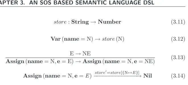
In order to evaluate both aVarand anAssignment we need a store. The store will represented using a function:

Store:Object→Object

A function consists of zero or more tuples, a tuple with a keyk and a value v

is written ask7→v. A concrete function withn tuples can be written as:

{k17

Operational Semantics Applied to Model Driven Engineering

T.J.L. Wolterink

Acknowledgements

Table of Contents

TABLE OF CONTENTS

List of Figures

List of Abbreviations

Introduction

1.2 Problem Statement

1.3 Research Objectives

1.4. CONTRIBUTIONS

1.4 Contributions

1.5 Outline

1.5. OUTLINE

Basic Concepts

Models and Metamodels

2.2. MODEL DRIVEN ENGINEERING

Model Definition

Metamodel Definition

2.3 MDE Approaches

MS Software Factory Tools

2.4. DOMAIN SPECIFIC LANGUAGES

Eclipse Modelling Framework

2.4 Domain Specific Languages

MetaModel

2.5 Semantics of Languages

2.5. SEMANTICS OF LANGUAGES

Approaches

2.6 Structural Operational Semantics

Rules

2.6. STRUCTURAL OPERATIONAL SEMANTICS

Example

Transition System Specification

SOS Styles

2.7. APPROACHES TO DEFINING THE SEMANTICS OF MODELLING LANGUAGES

2.7 Approaches to defining the Semantics of

Model Transformations

Graph Transformations

Simulation in the Topcased Toolkit

2.8. CONCLUSION

Semantic Anchoring

2.8 Conclusion

An SOS based Semantic Language DSL

3.2 SOS for Expressions

3.2. SOS FOR EXPRESSIONS

Semantics

3.2. SOS FOR EXPRESSIONS

Example Simulation

3.3 Introducing the Store

Semantics

3.3. INTRODUCING THE STORE