Abstract—The issue of modelling and forecasting the share prices of the banking sector remains a challenge because of high volatilities in individual stock prices. Reliably forecasting the future values of shares is essential to minimize the risk for investors, but there is currently no standard forecasting procedure or technique that can be used in modelling and forecasting the share prices of the banking sector. This research is concerned with the development of a forecasting algorithm that can be applied in modelling and forecasting the share prices of the banking sector. It proposes six steps that, when followed, may lead to obtaining superior models. These steps are Data Selection, Data Preparation, Training the Model, Refining the Model, Testing the Model, and Forecast Production. These building steps were used to build a forecasting model for HSBC Bank Plc. and Lloyds TSB using the Back-propagation Neural Network. Empirical results show that superior models were obtained by applying the proposed algorithm compared to the financial forecasting models published in the literature.
Index Terms—forecasting algorithm, financial forecasting, banking sector, neural network.
I. INTRODUCTION
Modelling and forecasting shares in the banking sector has received much attention in the finance literature because of the high volatilities in its prices which represents a systematic risk faced by investors who hold these shares in their market. This is because the prices in the market are affected by many factors such as the economic and political climate, company’s performance, supply and demand and investors’ behaviour in general. Many investors observe the market closely when they buy or sell shares because of the future uncertainty in the prices of the shares. Hence, reliably forecasting the future values of shares is essential to minimize the risk for the investors. While some approaches have been successful in modelling certain
Manuscript received March 22, 2007.
A. Rahou, PhD Student, Faculty of Advanced Technology, University of Glamorgan, CF37 1DL, UK, Tel: +44(0)1443 482262, Fax: +44(0)1443 482169, E-mail: [email protected]
Dr. H. Al-Madfai, Senior Lecturer, Faculty of Advanced Technology, University of Glamorgan, CF37 1DL, UK, E-mail: [email protected]
Prof. H. Coombs, Head of Accounting, Finance & Information Management Department, Business School, University of Glamorgan, CF37 1DL, UK, E-mail: [email protected]
D, Gilleland, Deposits Manager, Julian Hodge Bank Ltd., UK, E-mail: [email protected]
Prof. A. Ware, Head of Computing & Mathematical Sciences, Faculty of Advanced Technology, University of Glamorgan, CF37 1DL, UK, E-mail: [email protected]
datasets, the success of a forecasting model on a time series does not guarantee its success with another. Hence, there is no standard forecasting procedure or technique that can be used in modelling and forecasting the share prices of the banking sector.
One notable work attempting to address this issue is the algorithm proposed by Yao & Tan [10]. However, applying their proposed algorithm was not always enough to arrive at an adequate forecasting model. This may be because the proposed steps do not include feed-back and feed-forward mechanisms to update the input data or the forecasting approach used to build the forecasting model when an insufficiently accurate model is obtained.
This research is concerned with the development of a generalized forecasting algorithm that can be applied in modelling and forecasting the share prices of the banking sector.
II. PROPOSED ALGORITHM
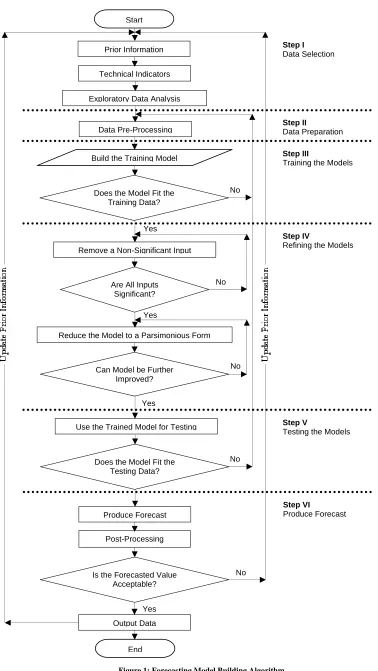
The flowchart of the proposed algorithm is given in Fig. 1. It can be seen from Fig. 1 that the algorithm consists of six steps, with feed-back and feed-forward loops. The following sections introduce the modelling and forecasting steps proposed by the algorithm.
A. Data Selection
The first step of the modelling and forecasting process is selecting, from the available data, the inputs to be used in building the forecasting model. All the relevant or possibly relevant data to the target should be investigated for possible inclusion. The most common data which is pertinent to the banking sector are the historic share prices, the factors that affect share prices, and the historic financial statements of the companies.
It is proposed that this step consists of three main stages, as follows:
1. Prior Information
Prior information refers to all the relevant information available at the beginning of the forecasting model building process. In addition to the related data which is mentioned above, prior information may include:
Available forecasting approaches that can be used to
forecast the share prices,
Available experience and knowledge, and
Available tools such as software and facilities.
A Generalized Algorithm for Modelling &
Forecasting the Share Prices of the Banking Sector
Figure 1: Forecasting Model Building Algorithm No
No No
Use the Trained Model for Testing
Step II
Data Preparation Exploratory Data Analysis
End
Step III
Training the Models
Step V
Testing the Models Step I
Data Selection
Is the Forecasted Value Acceptable?
Output Data Yes Does the Model Fit the
Testing Data? Start
Yes Data Pre-Processing
Does the Model Fit the Training Data? Prior Information
Technical Indicators
Build the Training Model
No
Step IV
Refining the Models
Step VI
Produce Forecast Produce Forecast
Post-Processing Remove a Non-Significant Input
Reduce the Model to a Parsimonious Form Are All Inputs
Significant?
Yes
No
Can Model be Further Improved?
Which of these to be used in modelling can be determined by using evidence from the literature and the analysts’ own experience.
2. Technical Indicators
Usually technical indicators are used to depict a time series, those with high volatility in their movements, by removing noise, outliers, and other sources of variation. In general, technical indicators re-assemble all the information that is derived by applying some mathematical transformations to the data in a time series. They can be useful in understanding the general movement of the time series.
For example, one important technical indicator in financial time series is turning points, generally defined as the changing points in the direction of the time series [2], [7] can be used as an input when building the forecasting model to help build improved forecasting models.
The binary turning point in period n variable can be
obtained from:
⎪
⎩
⎪
⎨
⎧
<
>
>
<
=
− − + ++ +
− −
otherwise
y
y
y
y
y
y
y
y
y
y
TP
t n t t t t nn t t
t t n t
t
0
,...,
,...,
1
,...,
,...,
1
1 1
1 1
where n is the turning points time window.
As there are two types of turning points, maxima and minima, where the maxima turning point is generated at
time t when there are lower values in each side of time t
while the minima turning point is generated at time t when
there are higher values in each side of time t.
Therefore, the type of turning point technical indicator
variable in period n can be obtained from:
⎪
⎩
⎪
⎨
⎧
<
>
−
>
<
+
=
− − + ++ +
− −
otherwise
y
y
y
y
y
y
y
y
y
y
TP
t n t t t t nn t t
t t n t
t
0
,...,
,...,
1
,...,
,...,
1
1 1
1 1
3. Exploratory Data Analysis
Exploratory data analysis (EDA) is an important step in time series analysis. It provides an exploration of the data before starting with the forecasting process. The first step of EDA is usually plotting the time series against time to obtain an overview of the dataset. This step is useful to identify anomalies such as missing data and outliers.
Other EDA techniques involve plotting the autocorrelation function (ACF) and partial autocorrelation function (PACF) to identify if the time series was seasonal and the periodicity of that seasonality.
B. Data Preparation
After collecting the data and prior to building the forecasting model, the data is usually subjected to several pre-processing operations. This is normally carried out to increase the quality of the data since the success of any forecasting model depends on the quality of the input data.
Common data preparation and pre-processing techniques include:
1. Linear Differencing
Linear differencing is a pre-processing technique which is used to measure the difference between the values in a time series separated by a specific time period. It is often used to remove the trend and seasonality in time series data [1].
First-order linear differencing is obtained by subtracting
the value at time t and the immediately preceding value at
time t-1 [7]. Analytically it is obtained from:
1
−
−
=
∇
y
ty
ty
t (1)Seasonal differencing is calculated by subtracting the
value at time t and the corresponding preceding value at
time t-s, according to the seasonal period [7], where s is the periodicity of the seasonal component of the data. Analytically it is obtained from:
n t t t
s
y
=
y
−
y
−∇
(2)Some studies refer to the differenced dataset as the “momentum” of the shares; see for example [11].
2. Normalization
Normalization is a pre-processing technique obtained using the standard deviation and the average of the dataset. It is useful to decrease the absolute range of the values of a time series.
For a given value
y
t , its normalized value can beobtained from:
SD
y
y
z
tt
−
=
(3)where,
y the mean value of the dataset
SD the standard deviation
Normalization often fails when the mean is unrepresentative of the data, such as when there is a linear trend in the time series.
3. Data Smoothing
Smoothing the data may be useful in understanding the fundamental trend of the data i.e. to reduce the noise and random components of the data.
Many methods can be used to smooth the data including the Crude Moving Average. This is an established and widely-used technique to smooth data [3], [4], [8].
In time series analysis there are two types of moving average; these are the centred moving average (CMA) and the prior moving average (PMA) [5], [7].
The main difference is that CMA is centred in the middle of the selected data, whilst the PMA is positioned next to the last number.
CMA for an odd number of observations is obtained from:
∑
−− −
= +
=
(( 1)/2)) 2 / ) 1 ((
1
nn j
j t
t
y
n
CMA
(4)where n is the moving average time window.
While the CMA for an even number of observations is obtained from:
(
)
⎟⎟
⎠
⎞
⎜⎜
⎝
⎛
+
−
=
∑
∑
+ −
= +
−
−
= +
) 2 / (
1 ) 2 / ( 1
) 2 / (
) 2 / (
1
2
1
nn j
j t n
n j
j t
t
y
y
n
CMA
(5)The PMA is obtained from:
∑
=
=
nt t
t
y
n
PMA
1
1
(6)
PMA is generally used to smooth time series data. This is because it depends only on the past observations while, by contrast, calculating the centred moving average depends on the past and future observations.
C. Training the Models
The initial stage of this process is to choose the size of the dataset required to train the model. It is generally, the case that a large proportion of the available data is used for training and the remaining smaller proportion is used for testing.
Model training is generally performed in two steps: the first step fits the model using the given inputs, and the second step verifies the validity of the model by comparing within sample forecasts to the observed values.
Training the model, in the case of using neural network for example, can be done using different types of input data employing different model architectures [6], [9]. Model architecture refers to the number of input layers, hidden layers and output layers which are used to build the forecasting model. While training the model using GARCH involves finding appropriate initial estimates of the parameters and then successively refines them until the optimum values of the parameters are obtained.
In general, when the forecasting model, which is obtained, gives unacceptable results, this leads to a revisiting of the data preparation step in order to choose a different set of inputs and possibly different model. This is usually iterated until improved results are obtained.
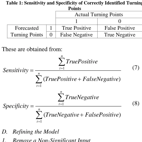
The most significant problem to avoid in this step is over-training and over-parameterization [7], [9]. To solve this problem, a decision has to be made as when the training should stop. The point at which training stops usually depends on the forecasting accuracy measures used. For example, novel accuracy measures such as sensitivity and specificity of predicted turning points may be used, in addition to the conventional least squares error, to evaluate the performance of the forecasting models and hence avoid this problem. In this instance, sensitivity refers to the
[image:4.612.321.556.123.357.2]percentage of correctly identified positive values to the total number of positive values, i.e. true positive, while the specificity refers to the percentage of correctly identified negative values to the total number of negative values, i.e. true negative, as shown in Table 1 below.
Table 1: Sensitivity and Specificity of Correctly Identified Turning Points
Actual Turning Points
1 0 Forecasted
Turning Points
1 True Positive False Positive 0 False Negative True Negative
These are obtained from:
∑
∑
=
=
+ =
n
t
n
t
ive FalseNegat ve
TruePositi
ve TruePositi y
Sensitivit
1
1
) (
(7)
) (
1
1
ive FalsePosit Negative
True
Negative True
y
Specificit n
t
n
t
+ =
∑
∑
=
= (8)
D. Refining the Model
1. Remove a Non-Significant Input
This step involves removing non-significant inputs, i.e. keeping the inputs that significantly affect the output and discarding the inputs that have smaller or no affect on the output. This can be done by removing inputs one at time and evaluating the performance of the model at each step.
2. Reduce the Model to a Parsimonious Form
This is an optimization of the number of parameters and accuracy measures, so that the model would have an optimum accuracy measure with as few parameters as possible.
E. Testing the Model
Testing the model is an attempt to investigate the forecasting capability of the trained model by using a time window of the time series that was not used in building the model [8], [9]. It is conventional that a small proportion of the data is usually used for testing.
Hence, this step entails checking the trained model to ascertain whether it fits the testing data or not. If not, that leads back to the data preparation step to follow the steps again until an adequate testing model is obtained [8].
F. Producing Forecasts
After obtaining an adequate forecasting model, it can be used now to forecast the future values of the share prices. In many cases, a post-processing step is applied to the forecasts in order to revert them back to the data’s original scale. This is why it is essential that all pre-processing methods are reversible.
forecasting model building steps are started again from the beginning with updated prior information. This process is iterated until acceptable forecasts are obtained.
III. APPLICATION
The algorithm proposed in this paper was used to build a forecasting model for the share prices of two companies in the banking sector.
The historic daily open share prices of HSBC Bank Plc.
and Lloyds TSB Bank which cover the period between 3rd
of July 2000 until 24th of June 2005, as shown in Fig. 2 and
Fig. 3 respectively, were used in this research. The aim was
to forecast the future share prices for one day-ahead using a Back-Propagation Neural Network.
The models were Univariate, built using only the historic
share prices without exogenous variables (1).
The type of turning point technical indicator variable for ‘n=1’ (introduces in section II.A.2) was investigated as input in this research. It was expected that using the turning points of the share prices as input helps to build improved forecasting models.
(1) Exogenous variables resemble for example, the evaluation of company’s activities and the factors that affect share prices.
[image:5.612.74.554.215.438.2]550 650 750 850 950 1050 1150 03/0 7/20 00 03/0 9/20 00 03/1 1/20 00 03/0 1/20 01 03/0 3/20 01 03/0 5/20 01 03/0 7/20 01 03/0 9/20 01 03/1 1/20 01 03/0 1/20 02 03/0 3/20 02 03/0 5/20 02 03/0 7/20 02 03/0 9/20 02 03/1 1/20 02 03/0 1/20 03 03/0 3/20 03 03/0 5/20 03 03/0 7/20 03 03/0 9/20 03 03/1 1/20 03 03/0 1/20 04 03/0 3/20 04 03/0 5/20 04 03/0 7/20 04 03/0 9/20 04 03/1 1/20 04 03/0 1/20 05 03/0 3/20 05 03/0 5/20 05 Date O pe n S ha re P ri c e s
Figure 2: The historic daily share prices of HSBC Bank Plc. which cover the period between 3rd of July 2000 until 24th of June 2005
250 350 450 550 650 750 850 03/0 7/2 000 03/0 9/2 000 03/1 1/2 000 03/0 1/2 001 03/0 3/2 001 03/0 5/2 001 03/0 7/2 001 03/0 9/2 001 03/1 1/2 001 03/0 1/2 002 03/0 3/2 002 03/0 5/2 002 03/0 7/2 002 03/0 9/2 002 03/1 1/2 002 03/0 1/2 003 03/0 3/2 003 03/0 5/2 003 03/0 7/2 003 03/0 9/2 003 03/1 1/2 003 03/0 1/2 004 03/0 3/2 004 03/0 5/2 004 03/0 7/2 004 03/0 9/2 004 03/1 1/2 004 03/0 1/2 005 03/0 3/2 005 03/0 5/2 005 Date O pe n S ha re P ri c e s
[image:5.612.70.555.461.686.2]A number of missing observations were identified through EDA. The missing data were estimated by taking the average of the two nearest good neighbours, as these are likely to be similar to the market conditions underlying the missing observations.
Share values in public holidays (2) were equated to the
close share prices of the previous trading day, so that
price close previous t
holiday
t
y
Y
ˆ
,=
−1, (9)The historic daily share prices of the case studies were normalized and pre-processed prior to including them as inputs to the forecasting models. The input data considered
were the share prices on the day (yt), share prices for one
day before (yt-1), share prices for two days before (yt-2),
share prices for three days before (yt-3), share prices for four
days before (yt-4), first order and second order differenced
data, and a number of moving average series obtained using different time windows.
The data used for training in this application covers the
period between 3rd of July 2000 until 31st of Dec. 2004.
For HSBC Bank Plc., an initial model was selected. This model had optimum maximum percentages of the sensitivity and specificity of the predicted turning points and Root Mean Square Error (RMSE), which were 50%, 51%, and 0.0345 respectively. This model was built using
13 inputs (yt-4, yt-3, yt-2, yt-1, yt, 5MAt(3), 10MAt, 20MAt,
(2) Public holidays include Christmas day, Easter day and bank holidays.
(3) The notation is that the window size of the moving average indicates the period of which the moving average is a summary of. For example, the moving average for one working week is denoted by (5MAt), while the
moving average for two working weeks is denoted by (10MAt), and so on.
40MAt, 60MAt, first-order differencing, Relative Strength Index (RSI) and binary turning points for ‘n=1’) and 14 neurons in one hidden layer.
In the refining step, the number of inputs was reduced to 12 after removing the non-significant input 60MAt and reducing the number of neurons to 9 in one hidden layer. The model, after refinement, yielded sensitivity of the predicted turning points of 55%, specificity of the predicted turning points of 54% and RMSE 0.0334.
The historic daily open share prices, covering the period
between 3rd of January 2005 until 24th of June 2005, were
used for testing the trained model. This resulted in sensitivity of the predicted turning points of 50%, specificity of the predicted turning points of 59% and RMSE 0.0189.
The model was rebuilt using the type of turning points instead of the binary turning points as input. The forecasts obtained from this model, shown in Fig. 4, yielded a one step-ahead sensitivity of predicted point of 63% and 77% for the training and testing, specificity of predicted turning points of 49% and 41% for the training and testing, and RMSE 0.0338 and 0.0236 for training and testing respectively.
To test the models, the forecasted share prices of 27th
June until 1st July 2005 were produced using the historic
data from 3rd July 2000 until 24th June 2005. To this end,
rolling forecast were produced, so that the actual share price
of 27th June 2005 was added to the input data to forecast the
share prices of 28th June 2005, and so on until the
forecasted share prices of 1st July 2005 was obtained. These
forecasts are shown in Table 2.
550 650 750 850 950 1050 1150
25/08 /20
00
25/10 /20
00
25/12 /20
00
25/0 2/20
01
25/0 4/20
01
25/06 /20
01
25/08 /20
01
25/ 10/
2001
25/1 2/20
01
25/ 02/
2002
25/04 /20
02
25/06 /20
02
25/0 8/20
02
25/1 0/2
002
25/ 12/
2002
25/02 /20
03
25/04 /20
03
25/0 6/20
03
25/08 /20
03
25/10 /20
03
25/12 /20
03
25/0 2/2
004
25/04 /20
04
25/06 /20
04
25/08 /20
04
25/10 /20
04
25/12 /20
04
Date
O
p
en
S
h
ar
e
P
ri
ces
[image:6.612.68.559.446.701.2]Actual Prices Forecasted Prices
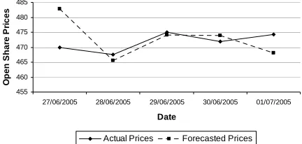
Table 2: Actual and forecast daily open share prices obtained for HSBC Bank Plc. in last week of June 2005
Date Actual Share
Prices
Forecasted Share Prices
27th June 2005 888.50 894.53
28th June 2005 888.00 891.26
29th June 2005 894.50 890.69
30th June 2005 889.00 888.09
[image:7.612.54.271.183.286.2]1st July 2005 893.00 876.84
Fig. 5 shows that the forecasting model produced forecasts in the same direction of the actual prices.
875 879 883 887 891 895 899
27/06/2005 28/06/2005 29/06/2005 30/06/2005 01/07/2005
Date
O
p
en
S
h
ar
e
Pr
ic
es
Actual Prices Forecasted Prices
Figure 5: Actual and genuine out of sample forecast daily open share prices for HSBC Bank Plc. for the last week of June 2005.
For Lloyds TSB Bank, an initial model was selected. This model had optimum maximum percentages of the sensitivity and specificity of the predicted turning points and RMSE as 57%, 49%, and 0.0402 respectively. This model was built using 11 inputs (yt-4, yt-3, yt-2, yt-1, yt, 5MAt, 10MAt, 20MAt, 40MAt, first-order differencing, and binary turning points for ‘n=1’) and 12 neurons in one hidden layer.
In the refining step, all the inputs were significant but the number of neurons in one hidden layer was reduced to 10. The model, after refinement, yielded sensitivity of the
predicted turning points of 62%, specificity of the predicted turning points of 52% and RMSE 0.0392.
The historic daily open share prices, covering the period
between 3rd of January 2005 until 24th of June 2005, were
used for testing the trained model. This resulted in sensitivity of the predicted turning points of 60%, specificity of the predicted turning points of 41% and RMSE 0.0340.
The model was rebuilt using the type of turning points instead of the binary turning points as input. The forecasts obtained from this model, shown in Fig. 6, yielded a one step-ahead sensitivity of predicted point of 70% and 71% for the training and testing, specificity of predicted turning points of 43% and 31% for the training and testing, and RMSE 0.0365 and 0.0203 for training and testing respectively.
To test the models, the forecasted share prices of 27th
June until 1st July 2005 were produced using the historic
data from 3rd July 2000 until 24th June 2005. To this end,
rolling forecast were produced, so that the actual share price
of 27th June 2005 was added to the input data to forecast the
share prices of 28th June 2005, and so on until the
forecasted share prices of 1st July 2005 was obtained. These
forecasts are shown in Table 3.
Table 3: Actual and forecast daily open share prices obtained for Lloyds TSB Bank in last week of June 2005
Date Actual Share
Prices
Forecasted Share Prices
27th June 2005 470.00 482.87
28th June 2005 467.50 465.54
29th June 2005 475.00 474.15
30th June 2005 472.00 473.85
1st July 2005 474.25 468.13
250 350 450 550 650 750 850
25/0 8/20
00
25/1 0/20
00
25/1 2/2
000
25/0 2/20
01
25/0 4/200
1
25/0 6/200
1
25/0 8/20
01
25/1 0/20
01
25/1 2/2
001
25/0 2/200
2
25/0 4/200
2
25/0 6/200
2
25/0 8/20
02
25/1 0/200
2
25/1 2/200
2
25/0 2/200
3
25/0 4/2
003
25/0 6/20
03
25/0 8/20
03
25/1 0/200
3
25/1 2/200
3
25/0 2/2
004
25/0 4/200
4
25/0 6/200
4
25/0 8/20
04
25/1 0/20
04
25/1 2/2
004
Date
O
p
en
S
h
ar
e
P
ri
ce
s
[image:7.612.58.557.414.690.2]Actual Prices Forecasted Prices
Fig. 7 shows that the forecasting model produced forecasts in the same direction of the actual prices.
455 460 465 470 475 480 485
27/06/2005 28/06/2005 29/06/2005 30/06/2005 01/07/2005
Date
O
p
en
S
h
ar
e P
ri
c
es
Actual Prices Forecasted Prices
Figure7: Actual and genuine out of sample forecast daily open share prices for Lloyds TSB Bank for the last week of June 2005.
The forecasting process requires generating the turning point of the last day of the used historic data in preference to using any exogenous variables. This is because the turning point of the last day of the used input data is unknown. In this application, this was done by simulating the experts’ opinion to use it as input when forecasting the future share prices. Hence, simulated turning points generated using the binomial and trinomial distributions with parameters based on the observed percentages of the turning points were used. Then these generated turning points, which resemble the last day of the used input data, were added to the available data to forecast the next day’s share price.
In general, forecasting process of the open share prices for one day-ahead has to be done early enough to buy or sell before the market closes as otherwise any price movements will already have taken place when the market opens in the next day.
IV. CONCLUSIONS
The overall results provide evidence suggesting that superior models, compared to the models published in the literature, to forecast the daily open share prices of the banking sector share prices may be obtained using the proposed algorithm. The feed-back and feed-forward mechanisms proposed in the algorithm did help in building
an adequate model to forecast the share prices of the banking sector. These mechanisms are used to update:
The per-processing of the data when obtaining
insufficient model from training and testing steps.
The prior information when obtaining unacceptable
forecasts.
Empirical results presented in this research give sufficient evidence to conclude that using the type of turning points variables as inputs generally yields superior forecasting models for datasets from the banking sector.
Using the accuracy measure (sensitivity and specificity of predicted turning points), in addition to the RMSE, did improve the model selection process.
This work may be further improved through using exogenous variables to determine the type of turning point for the last day of time series in stead of simulating the turning points using the binomial and trinomial distributions. It is expected that this could lead to improved forecasts in the banking sector.
REFERENCES
[1] Chatfield, C., The analysis of time series, an introduction, 1996. 5th
Edition. Chapman and Hall, London.
[2] Farnum, N. R. and L. W. Stanton, Qualitative forecasting methods, 1989. PWS-KENT publishing company, Boston.
[3] Gately, Edward J., Neural networks for financial forecasting, 1996. John Wiley & Sons Ltd.
[4] Jarrett, Jeffrey, Business forecasting methods, 1987. 1st Published, Basil Blackwell Ltd.
[5] Johnston, R. and M. G. Hagen and K. H. Jamieson, Priming and
persuasion in the 2000 presidential campaign, 2003. Annual meeting
of the Midwest political science association, Chicago, Illinois. [6] Lawrence, R., Using neural networks to forecast stock market prices,
1997. Department of computer science, University of Manitoba. [7] Makridakis, S. and S. C. Wheelwright and R. J. Hyndman,
Forecasting, methods and applications, 1998. John Wiley & Sons,
Inc. 3rd Edition.
[8] Pyle, D., Data preparation for data mining, 1999. Morgan Kaufmann Publishers, United States of America.
[9] Tarassenko, L., A guide to neural computing application, 1998. 1st
Published by Arnold, a member of the Hodder Headline Group. Co-published by John Wiley & Sons Inc.
[10] Yao, J. and C. L. TAN, Guidelines for financial forecasting with
neural networks. Proceedings of international conference on neural
information processing, Shanghai, China, 2001. P.757-761.
[11] Yao, J. and Hean-Lee P., Forecasting the KLSE Index using neural
networks. IEEE international conference on neural networks, Perth,