Learning Dictionaries for Named Entity Recognition using Minimal
Supervision
Arvind Neelakantan
Department of Computer Science University of Massachusetts, Amherst
Amherst, MA, 01003
Michael Collins
Department of Computer Science Columbia University New-York, NY 10027, USA
Abstract
This paper describes an approach for au-tomatic construction of dictionaries for Named Entity Recognition (NER) using large amounts of unlabeled data and a few seed examples. We use Canonical Cor-relation Analysis (CCA) to obtain lower dimensional embeddings (representations) for candidate phrases and classify these phrases using a small number of labeled examples. Our method achieves 16.5% and 11.3% F-1 score improvement over co-training on disease and virus NER re-spectively. We also show that by adding candidate phrase embeddings as features in a sequence tagger gives better perfor-mance compared to using word embed-dings.
1 Introduction
Several works (e.g., Ratinov and Roth, 2009; Co-hen and Sarawagi, 2004) have shown that inject-ing dictionary matches as features in a sequence tagger results in significant gains in NER perfor-mance. However, building these dictionaries re-quires a huge amount of human effort and it is of-ten difficult to get good coverage for many named entity types. The problem is more severe when we consider named entity types such as gene, virus and disease, because of the large (and growing) number of names in use, the fact that the names are heavily abbreviated and multiple names are used to refer to the same entity (Leaman et al., 2010; Dogan and Lu, 2012). Also, these dictionaries can only be built by domain experts, making the pro-cess very expensive.
This paper describes an approach for automatic construction of dictionaries for NER using large
amounts of unlabeled data and a small number of seed examples. Our approach consists of two steps. First, we collect a high recall, low preci-sion list ofcandidate phrasesfrom the large unla-beled data collection for every named entity type using simple rules. In the second step, we con-struct an accurate dictionary of named entities by removing the noisy candidates from the list ob-tained in the first step. This is done by learning a classifier using the lower dimensional, real-valued CCA (Hotelling, 1935) embeddings of the can-didate phrases as features and training it using a small number of labeled examples. The classifier we use is a binary SVM which predicts whether a candidate phrase is a named entity or not.
We compare our method to a widely used semi-supervised algorithm based on co-training (Blum and Mitchell, 1998). The dictionaries are first evaluated on virus (GENIA, 2003) and disease (Dogan and Lu, 2012) NER by using them directly in dictionary based taggers. We also give results comparing the dictionaries produced by the two semi-supervised approaches with dictionaries that are compiled manually. The effectiveness of the dictionaries are also measured by injecting dictio-nary matches as features in a Conditional Random Field (CRF) based tagger. The results indicate that our approach with minimal supervision pro-duces dictionaries that are comparable to dictio-naries compiled manually. Finally, we also com-pare the quality of the candidate phrase embed-dings with word embedembed-dings (Dhillon et al., 2011) by adding them as features in a CRF based se-quence tagger.
2 Background
We first give background on Canonical Correla-tion Analysis (CCA), and then give background on
CRFs for the NER problem.
2.1 Canonical Correlation Analysis (CCA) The input to CCA consists of n paired observa-tions(x1, z1), . . . ,(xn, zn)wherexi ∈ Rd1, zi ∈ Rd2 (∀i∈ {1,2, . . . , n})are the feature
represen-tations for the two views of a data point. CCA simultaneously learns projection matrices Φ1 ∈ Rd1×k,Φ2 ∈ Rd2×k (kis a small number) which
are used to obtain the lower dimensional represen-tations(¯x1,z¯1), . . . ,(¯xn,z¯n)wherex¯i = ΦT1xi ∈ Rk,z¯i = ΦT
2zi ∈Rk, ∀i∈ {1,2, . . . , n}. Φ1,Φ2 are chosen to maximize the correlation betweenx¯i andz¯i, ∀i∈ {1,2, . . . , n}.
Consider the setting where we have a label for the data point along with it’s two views and ei-ther view is sufficient to make accurate predic-tions. Kakade and Foster (2007) and Sridharan and Kakade (2008) give strong theoretical guaran-tees when the lower dimensional embeddings from CCA are used for predicting the label of the data point. This setting is similar to the one considered in co-training (Collins and Singer, 1999) but there is no assumption of independence between the two views of the data point. Also, it is an exact al-gorithm unlike the alal-gorithm given in Collins and Singer (1999). Since we are using lower dimen-sional embeddings of the data point for prediction, we can learn a predictor with fewer labeled exam-ples.
2.2 CRFs for Named Entity Recognition CRF based sequence taggers have been used for a number of NER tasks (e.g., McCallum and Li, 2003) and in particular for biomedical NER (e.g., McDonald and Pereira, 2005; Burr Settles, 2004) because they allow a great deal of flexibility in the features which can be included. The input to a CRF tagger is a sentence (w1, w2, . . . , wn) where wi, ∀i∈ {1,2, . . . , n}are words in the sentence. The output is a sequence of tags y1, y2, . . . , yn whereyi ∈ {B, I, O}, ∀i ∈ {1,2, . . . , n}. B is the tag given to the first word in a named entity,
Iis the tag given to all words except the first word in a named entity andOis the tag given to all other words. We used the standard NER baseline fea-tures (e.g., Dhillon et al., 2011; Ratinov and Roth, 2009) which include:
• Current Word wi and its lexical features which include whether the word is capital-ized and whether all the characters are
cap-italized. Prefix and suffixes of the word wi were also added.
• Word tokens in window of size two
around the current word which include wi−2, wi−1, wi+1, wi+2 and also the capital-ization pattern in the window.
• Previous two predictionsyi−1andyi−2.
The effectiveness of the dictionaries are evaluated by adding dictionary matches as features along with the baseline features (Ratinov and Roth, 2009; Cohen and Sarawagi, 2004) in the CRF tag-ger. We also compared the quality of the candi-date phrase embeddings with the word-level em-beddings by adding them as features (Dhillon et al., 2011) along with the baseline features in the CRF tagger.
3 Method
This section describes the two steps in our ap-proach: obtaining candidate phrases and classify-ing them.
3.1 Obtaining Candidate Phrases
We used the full text of 110,369 biomedical pub-lications in the BioMed Central corpus1to get the
high recall, low precision list of candidate phrases. The advantages of using this huge collection of publications are obvious: almost all (including rare) named entities related to the biomedical do-main will be mentioned and contains more re-cent developments than a structured resource like Wikipedia. The challenge however is that these publications are unstructured and hence it is a dif-ficult task to construct accurate dictionaries using them with minimal supervision.
The list of virus candidate phrases were ob-tained by extracting phrases that occur between “the” and “virus” in the simple pattern “the ... virus” during a single pass over the unlabeled doc-ument collection. This noisy list had a lot of virus names such asinfluenza,human immunodeficiency andEpstein-Barr along with phrases that are not virus names, likemutant,same,new, and so on.
to obtain the noisy list of disease names. We lected every sentence in the unlabeled data col-lection that has the word “disease” in it and ex-tracted noun phrases2 following the patterns
“dis-eases like ....”, “dis“dis-eases such as ....” , “dis“dis-eases in-cluding ....” , “diagnosed with ....”, “patients with ....” and “suffering from ....”.
3.2 Classification of Candidate Phrases Having found the list of candidate phrases, we now describe how noisy words are filtered out from them. We gather (spelling,context) pairs for every instance of a candidate phrase in the unla-beled data collection. spelling refers to the can-didate phrase itself while context includes three words each to the left and the right of the candidate phrase in the sentence. Thespellingand the con-textof the candidate phrase provide a natural split into two views which multi-view algorithms like co-training and CCA can exploit. The only super-vision in our method is to provide a few spelling seed examples (10 in the case of virus, 18 in the case of disease), for example,human immunodefi-ciencyis a virus andmutantis not a virus.
3.2.1 Approach using CCA embeddings We use CCA described in the previous section to obtain lower dimensional embeddings for the candidate phrases using the (spelling, context) views. Unlike previous works such as Dhillon et al. (2011) and Dhillon et al. (2012), we use CCA to learn embeddings for candidate phrases instead of all words in the vocabulary so that we don’t miss named entities which have two or more words.
Let the number of (spelling,context) pairs ben (sum of total number of instances of every can-didate phrase in the unlabeled data collection). First, we map the spelling and context to high-dimensional feature vectors. For thespellingview, we define a feature for every candidate phrase and also a boolean feature which indicates whether the phrase is capitalized or not. For thecontextview, we use features similar to Dhillon et al. (2011) where a feature for every word in the context in conjunction with its position is defined. Each of the n (spelling, context) pairs are mapped to a pair of high-dimensional feature vectors to get n paired observations (x1, z1), . . . ,(xn, zn) with xi ∈ Rd1, zi ∈ Rd2, ∀i ∈ {1,2, . . . , n}(d1, d2 are the feature space dimensions of the spelling 2Noun phrases were obtained using http://www.umiacs.umd.edu/ hal/TagChunk/
andcontextview respectively). Using CCA3, we
learn the projection matrices Φ1 ∈ Rd1×k,Φ2 ∈ Rd2×k (k << d1 and k << d2 ) and obtain
spellingview projectionsx¯i = ΦT1xi ∈ Rk,∀i∈
{1,2, . . . , n}. The k-dimensional spelling view projection of any instance of a candidate phrase is used as it’s embedding4.
The k-dimensional candidate phrase embed-dings are used as features to learn a binary SVM with the seedspellingexamples given in figure 1 as training data. The binary SVM predicts whether a candidate phrase is a named entity or not. Since the value of k is small, a small number of labeled examples are sufficient to train an accurate clas-sifier. The learned SVM is used to filter out the noisy phrases from the list of candidate phrases obtained in the previous step.
To summarize, our approach for classifying candidate phrases has the following steps:
• Input: n (spelling, context) pairs, spelling seed examples.
• Each of the n (spelling, context) pairs are mapped to a pair of high-dimensional fea-ture vectors to get n paired observations
(x1, z1), . . . ,(xn, zn) with xi ∈ Rd1, zi ∈ Rd2, ∀i∈ {1,2, . . . , n}.
• Using CCA, we learn the projection matri-ces Φ1 ∈ Rd1×k,Φ2 ∈ Rd2×k and ob-tainspellingview projections x¯i = ΦT1xi ∈ Rk,∀i∈ {1,2, . . . , n}.
• The embedding of a candidate phrase is given by the k-dimensional spelling view projec-tion of any instance of the candidate phrase.
• We learn a binary SVM with the candi-date phrase embeddings as features and the spelling seed examples given in figure 1 as training data. Using this SVM, we predict whether a candidate phrase is a named entity or not.
3.2.2 Approach based on Co-training
We discuss here briefly the DL-CoTrain algorithm (Collins and Singer, 1999) which is based on co-training (Blum and Mitchell, 1998), to classify 3Similar to Dhillon et al. (2012) we used the method given in Halko et al. (2011) to perform the SVD computation in CCA for practical considerations.
• Virus seedspelling examples
– Virus Names: human immunodeficiency, hepatitis C, influenza, Epstein-Barr, hepatitis B – Non-virus Names: mutant, same, wild type, parental, recombinant
• Disease seedspellingexamples
– Disease Names: tumor, malaria, breast cancer, cancer, IDDM, DM, A-T, tumors, VHL – Non-disease Names: cells, patients, study, data, expression, breast, BRCA1, protein, mutant
1
Figure 1: Seedspellingexamples
candidate phrases. We compare our approach us-ing CCA embeddus-ings with this approach. Here, two decision list of rules are learned simultane-ously one using the spelling view and the other using the context view. The rules using the spellingview are of the form: full-string=human immunodeficiency→Virus, full-string=mutant→
Not a virus and so on. In the context view, we used bigram5 rules where we considered all
pos-sible bigrams using the context. The rules are of two types: one which gives a positive label, for example, full-string=human immunodeficiency→
Virus and the other which gives a negative label, for example, full-string=mutant → Not a virus. The DL-CoTrain algorithm is as follows:
• Input: (spelling, context) pairs for every in-stance of a candidate phrase in the corpus,m specifying the number of rules to be added in every iteration, precision threshold,spelling seed examples.
• Algorithm:
1. Initialize the spellingdecision list using thespellingseed examples given in fig-ure 1 and seti= 1.
2. Label the entire input collection using the learned decision list ofspellingrules. 3. Add i ×m new context rules of each
type to the decision list of contextrules using the current labeled data. The rules are added using the same criterion as given in Collins and Singer (1999), i.e., among the rules whose strength is greater than the precision threshold , the ones which are seen more often with the corresponding label in the input data collection are added.
5We tried using unigram rules but they were very weak predictors and the performance of the algorithm was poor when they were considered.
4. Label the entire input collection using the learned decision list ofcontextrules. 5. Add i×m new spelling rules of each
type to the decision list ofspellingrules using the current labeled data. The rules are added using the same criterion as in step 3. Seti=i+1. If rules were added in the previous iteration, return to step 2.
The algorithm is run until no new rules are left to be added. The spelling decision list along with its strength (Collins and Singer, 1999) is used to construct the dictionaries. The phrases present in thespellingrules which give a positive label and whose strength is greater than the precision thresh-old, were added to the dictionary of named enti-ties. We found the parameters m and difficult to tune and they could significantly affect the per-formance of the algorithm. We give more details regarding this in the experiments section.
4 Related Work
Previously, Collins and Singer (1999) introduced a multi-view, semi-supervised algorithm based on co-training (Blum and Mitchell, 1998) for collect-ing names of people, organizations and locations. This algorithm makes a strong independence as-sumption about the data and employs many heuris-tics to greedily optimize an objective function. This greedy approach also introduces new param-eters that are often difficult to tune.
abbreviations (Kazama and Torisawa, 2007). For example, DM is the abbreviation for the disease Diabetes Mellitusand the disambiguation page for DMin Wikipedia associates it to more than 50 cat-egories since DM can be expanded to Doctor of Management,Dichroic mirror, and so on, each of it belonging to a different category. Due to the rapid growth of Wikipedia, the number of enti-ties that have disambiguation pages is growing fast and it is increasingly difficult to retrieve the article we want. Also, it is tough to understand these ap-proaches from a theoretical standpoint.
Dhillon et al. (2011) used CCA to learn word embeddings and added them as features in a se-quence tagger. They show that CCA learns bet-ter word embeddings than CW embeddings (Col-lobert and Weston , 2008), Hierarchical log-linear (HLBL) embeddings (Mnih and Hinton, 2007) and embeddings learned from many other tech-niques for NER and chunking. Unlike PCA, a widely used dimensionality reduction technique, CCA is invariant to linear transformations of the data. Our approach is motivated by the theoreti-cal result in Kakade and Foster (2007) which is developed in the co-training setting. We directly use the CCA embeddings to predict the label of a data point instead of using them as features in a sequence tagger. Also, we learn CCA embed-dings for candidate phrases instead of all words in the vocabulary since named entities often contain more than one word. Dhillon et al. (2012) learn a multi-class SVM using the CCA word embed-dings to predict the POS tag of a word type. We extend this technique to NER by learning a binary SVM using the CCA embeddings of a high recall, low precision list of candidate phrases to predict whether a candidate phrase is a named entity or not.
5 Experiments
In this section, we give experimental results on virus and disease NER.
5.1 Data
The noisy lists of both virus and disease names were obtained from the BioMed Central corpus. This corpus was also used to get the collection of (spelling,context) pairs which are the input to the CCA procedure and the DL-CoTrain algorithm de-scribed in the previous section. We obtained CCA embeddings for the 100,000most frequently
oc-curring word types in this collection along with every word type present in the training and de-velopment data of the virus and the disease NER dataset. These word embeddings are similar to the ones described in Dhillon et al. (2011) and Dhillon et al. (2012).
We used the virus annotations in the GE-NIA corpus (GEGE-NIA, 2003) for our experiments. The dataset contains 18,546 annotated sentences. We randomly selected 8,546 sentences for train-ing and the remaintrain-ing sentences were randomly split equally into development and testing sen-tences. The training sentences are used only for experiments with the sequence taggers. Previ-ously, Zhang et al. (2004) tested their HMM-based named entity recognizer on this data. For disease NER, we used the recent disease corpus (Dogan and Lu, 2012) and used the same training, devel-opment and test data split given by them. We used a sentence segmenter6 to get sentence segmented
data and Stanford Tokenizer7to tokenize the data.
Similar to Dogan and Lu (2012), all the different disease categories were flattened into one single category of disease mentions. The development data was used to tune the hyperparameters and the methods were evaluated on the test data.
5.2 Results using a dictionary-based tagger First, we compare the dictionaries compiled us-ing different methods by usus-ing them directly in a dictionary-based tagger. This is a simple and informative way to understand the quality of the dictionaries before using them in a CRF-tagger. Since these taggers can be trained using a hand-ful of training examples, we can use them to build NER systems even when there are no labeled sen-tences to train. The input to a dictionary tagger is a list of named entities and a sentence. If there is an exact match between a phrase in the input list to the words in the given sentence then it is tagged as a named entity. All other words are labeled as non-entities. We evaluated the performance of the following methods for building dictionaries:
• Candidate List: This dictionary contains all the candidate phrases that were obtained us-ing the method described in Section 3.1. The noisy list of virus candidates and disease can-didates had 3,100 and 60,080 entries respec-tively.
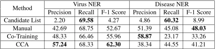
Method Precision Recall F-1 Score Precision Recall F-1 ScoreVirus NER Disease NER
Candidate List 2.20 69.58 4.27 4.86 60.32 8.99
Manual 42.69 68.75 52.67 51.39 45.08 48.03
Co-Training 48.33 66.46 55.96 58.87 23.17 33.26
[image:6.595.113.488.62.147.2]CCA 57.24 68.33 62.30 38.34 44.55 41.21 Table 1: Precision, recall, F- 1 scores of dictionary-based taggers
• Manual: Manually constructed dictionaries, which requires a large amount of human ef-fort, are employed for the task. We used the list of virus names given in Wikipedia8.
Un-fortunately, abbreviations of virus names are not present in this list and we could not find any other more complete list of virus names. Hence, we constructed abbreviations by con-catenating the first letters of all the strings in a virus name, for every virus name given in the Wikipedia list.
For diseases, we used the list of disease names given in the Unified Medical Lan-guage System (UMLS) Metathesaurus. This dictionary has been widely used in disease NER (e.g., Dogan and Lu, 2012; Leaman et al., 2010)9.
• Co-Training: The dictionaries are con-structed using the DL-CoTrain algorithm de-scribed previously. The parameters used werem= 5and= 0.95as given in Collins and Singer (1999). The phrases present in thespellingrules which give a positive label and whose strength is greater than the preci-sion threshold, were added to the dictionary of named entities.
In our experiment to construct a dictionary of virus names, the algorithm stopped after just 12 iterations and hence the dictionary had only 390 virus names. This was because there were no spelling rules with strength greater than 0.95 to be added. We tried varying both the parameters but in all cases, the algo-rithm did not progress after a few iterations. We adopted a simple heuristic to increase the coverage of virus names by using the strength of thespellingrules obtained after the12th it-eration. Allspellingrules that give a positive 8http://en.wikipedia.org/wiki/List of viruses
9The list of disease names from UMLS can be found at https://sites.google.com/site/fmchowdhury2/bioenex .
label and which has a strength greater than θwere added to the decision list ofspelling rules. The phrases present in these rules are added to the dictionary. We picked theθ pa-rameter from the set [0.1, 0.2, 0.3, 0.4, 0.5, 0.6, 0.7, 0.8, 0.9] using the development data. The co-training algorithm for constructing the dictionary of disease names ran for close to 50 iterations and hence we obtained bet-ter coverage for disease names. We still used the same heuristic of adding more named en-tities using the strength of the rule since it performed better.
• CCA: Using the CCA embeddings of the candidate phrases10 as features we learned a
binary SVM11to predict whether a candidate
phrase is a named entity or not. We consid-ered using 10 to 30 dimensions of candidate phrase embeddings and the regularizer was picked from the set [0.0001, 0.001, 0.01, 0.1, 1, 10, 100]. Both the regularizer and the num-ber of dimensions to be used were tuned us-ing the development data.
Table 1 gives the results of the dictionary based taggers using the different methods described above. As expected, when the noisy list of candi-date phrases are used as dictionaries the recall of the system is quite high but the precision is very low. The low precision of the Wikipedia virus lists was due to the heuristic used to obtain ab-breviations which produced a few noisy abbrevia-tions but this heuristic was crucial to get a high re-call. The list of disease names from UMLS gives a low recall because the list does not contain many disease abbreviations and composite disease men-tions such asbreast and ovarian cancer. The pres-10The performance of the dictionaries learned from word embeddings was very poor and we do not report it’s perfor-mance here.
0 1000 2000 3000 4000 5000 6000 7000 8000 9000 0.5
0.55 0.6 0.65 0.7 0.75 0.8 0.85
Number of Training Sentences
F−1 Score
Virus NER
baseline manual co−training cca
0 1000 2000 3000 4000 5000 6000
0.45 0.5 0.55 0.6 0.65 0.7 0.75 0.8
F−1 Score
Number of Training Sentences
Disease NER
baseline manual co−training cca
[image:7.595.78.517.71.247.2]1
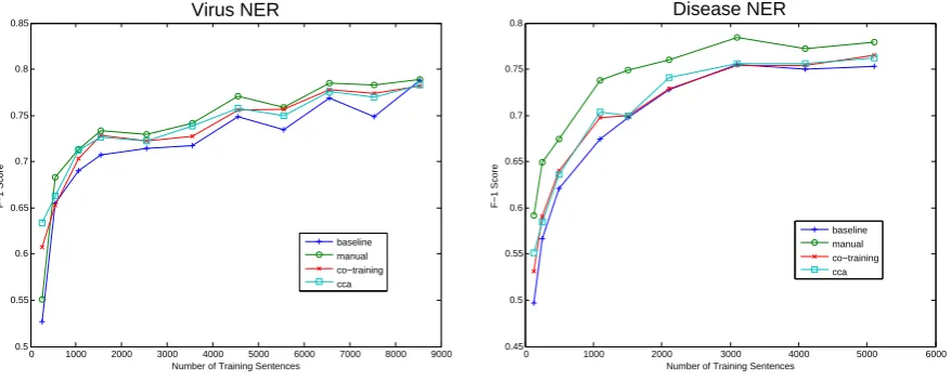
Figure 2: Virus and Disease NER F-1 scores for varying training data size when dictionaries obtained from different methods are injected
ence of ambiguous abbreviations affected the ac-curacy of this dictionary.
The virus dictionary constructed using the CCA embeddings was very accurate and the false pos-itives were mainly due to ambiguous phrases, for example, in the phrase HIV replication, HIV which usually refers to the name of a virus is tagged as a RNA molecule. The accuracy of the disease dictionary produced using CCA embed-dings was mainly affected by noisy abbreviations. We can see that the dictionaries obtained us-ing CCA embeddus-ings perform better than the dic-tionaries obtained from co-training on both dis-ease and virus NER even after improving the co-training algorithm’s coverage using the heuristic described in this section. It is important to note that the dictionaries constructed using the CCA embeddings and a small number of labeled exam-ples performs competitively with dictionaries that are entirely built by domain experts. These re-sults show that by using the CCA based approach we can build NER systems that give reasonable performance even for difficult named entity types with almost no supervision.
5.3 Results using a CRF tagger
We did two sets of experiments using a CRF tag-ger. In the first experiment, we add dictionary fea-tures to the CRF tagger while in the second ex-periment we add the embeddings as features to the CRF tagger. The same baseline model is used in both the experiments whose features are described
in Section 2.2. For both the CRF12 experiments
the regularizers from the set [0.0001, 0.001, 0.01, 0.1, 1.0, 10.0] were considered and it was tuned on the development set.
5.3.1 Dictionary Features
Here, we inject dictionary matches as features (e.g., Ratinov and Roth, 2009; Cohen and Sarawagi, 2004) in the CRF tagger. Given a dic-tionary of named entities, every word in the input sentence has a dictionary feature associated with it. When there is an exact match between a phrase in the dictionary with the words in the input sen-tence, the dictionary feature of the first word in the named entity is set toBand the dictionary fea-ture of the remaining words in the named entity is set toI. The dictionary feature of all the other words in the input sentence which are not part of any named entity in the dictionary is set toO. The effectiveness of the dictionaries constructed from various methods are compared by adding dictio-nary match features to the CRF tagger. These dic-tionary match features were added along with the baseline features.
0 1000 2000 3000 4000 5000 6000 7000 8000 9000 0.5
0.55 0.6 0.65 0.7 0.75 0.8 0.85
F−1 Score
Number of Training Sentences
Virus NER
baseline cca−word cca−phrase
0 1000 2000 3000 4000 5000 6000
0.45 0.5 0.55 0.6 0.65 0.7 0.75 0.8
Number of Training Sentences
F−1 Score
Disease NER
baseline cca−word cca−phrase
[image:8.595.79.517.71.247.2]1
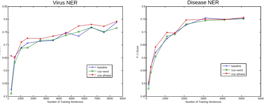
Figure 3: Virus and Disease NER F-1 scores for varying training data size when embeddings obtained from different methods are used as features
previously, the dictionaries produced from our ap-proach performs competitively with dictionaries that are entirely built by domain experts.
5.3.2 Embedding Features
The quality of the candidate phrase embeddings are compared with word embeddings by adding the embeddings as features in the CRF tagger. Along with the baseline features, CCA-word model adds word embeddings as features while the CCA-phrase model adds candidate phrase em-beddings as features.CCA-wordmodel is similar to the one used in Dhillon et al. (2011).
We considered adding 10, 20, 30, 40 and 50 di-mensional word embeddings as features for every training data size and the best performing model on the development data was picked for the exper-iments on the test data. For candidate phrase em-beddings we used the same number of dimensions that was used for training the SVMs to construct the best dictionary.
When candidate phrase embeddings are ob-tained using CCA, we do not have embeddings for words which are not in the list of candidate phrases. Also, a candidate phrase having more than one word has a joint representation, i.e., the phrase “human immunodeficiency” has a lower dimensional representation while the words “hu-man” and “immunodeficiency” do not have their own lower dimensional representations (assuming they are not part of the candidate list). To over-come this issue, we used a simple technique to dif-ferentiate between candidate phrases and the rest
of the words. Letxbe the highest real valued can-didate phrase embedding and the cancan-didate phrase embedding be addimensional real valued vector. If a candidate phrase occurs in a sentence, the em-beddings of that candidate phrase are added as fea-tures to the first word of that candidate phrase. If the candidate phrase has more than one word, the other words in the candidate phrase are given an embedding of dimension d with each dimension having the value2×x. All the other words are given an embedding of dimensiondwith each di-mension having the value4×x.
Figure 3 shows that almost always the candi-date phrase embeddings help the CRF model. It is also interesting to note that sometimes the word-level embeddings have an adverse affect on the performance of the CRF model. TheCCA-phrase model performs significantly better than the other two models when there are fewer labeled sen-tences to train and the separation of the candidate phrases from the other words seems to have helped the CRF model.
6 Conclusion
Acknowledgments
We are grateful to Alexander Rush, Alexandre Passos and the anonymous reviewers for their useful feedback. This work was supported by the Intelligence Advanced Research Projects Ac-tivity (IARPA) via Department of Interior Na-tional Business Center (DoI/NBC) contract num-ber D11PC20153. The U.S. Government is autho-rized to reproduce and distribute reprints for Gov-ernmental purposes notwithstanding any copy-right annotation thereon. The views and conclu-sions contained herein are those of the authors and should not be interpreted as necessarily represent-ing the official policies or endorsements, either ex-pressed or implied, of IARPA, DoI/NBC, or the U.S. Government.
References
Andrew McCallum and Wei Li. Early Results for Named Entity Recognition with Conditional Ran-dom Fields, Feature Induction and Web-Enhanced Lexicons. 2003. Conference on Natural Language Learning (CoNLL).
Andriy Mnih and Geoffrey Hinton.Three New Graph-ical Models for StatistGraph-ical Language Modelling. 2007. International Conference on Machine learn-ing (ICML).
Antonio Toral and Rafael Mu˜noz. A proposal to auto-matically build and maintain gazetteers for Named Entity Recognition by using Wikipedia. 2006. Workshop On New Text Wikis And Blogs And Other Dynamic Text Sources.
Avrin Blum and Tom M. Mitchell.Combining Labeled and Unlabeled Data with Co-Training. 1998. Con-ference on Learning Theory (COLT).
Burr Settles. Biomedical Named Entity Recognition Using Conditional Random Fields and Rich Feature Sets. 2004. International Joint Workshop on Natural Language Processing in Biomedicine and its Appli-cations (NLPBA).
H. Hotelling. Canonical correlation analysis (cca) 1935. Journal of Educational Psychology.
Jie Zhang, Dan Shen, Guodong Zhou, Jian Su and Chew-Lim Tan. Enhancing HMM-based Biomed-ical Named Entity Recognition by Studying Special Phenomena. 2004. Journal of Biomedical Informat-ics.
Jin-Dong Kim, Tomoko Ohta, Yuka Tateisi and Jun’ichi Tsujii. GENIA corpus - a semantically an-notated corpus for bio-textmining.2003. ISMB.
Junichi Kazama and Kentaro Torisawa. Exploiting Wikipedia as External Knowledge for Named Entity Recognition. 2007. Association for Computational Linguistics (ACL).
Karthik Sridharan and Sham M. Kakade. An Informa-tion Theoretic Framework for Multi-view Learning. 2008. Conference on Learning Theory (COLT). Lev Ratinov and Dan Roth. Design Challenges
and Misconceptions in Named Entity Recognition. 2009. Conference on Natural Language Learning (CoNLL).
Michael Collins and Yoram Singer. Unsupervised Models for Named Entity Classification. 1999. In Proceedings of the Joint SIGDAT Conference on Empirical Methods in Natural Language Processing and Very Large Corpora.
Nathan Halko, Per-Gunnar Martinsson, Joel A. Tropp. Finding structure with randomness: Probabilistic algorithms for constructing approximate matrix de-compositions. 2011. Society for Industrial and Ap-plied Mathematics.
Paramveer S. Dhillon, Dean Foster and Lyle Ungar. Multi-View Learning of Word Embeddings via CCA. 2011. Advances in Neural Information Processing Systems (NIPS).
Paramveer Dhillon, Jordan Rodu, Dean Foster and Lyle Ungar. Two Step CCA: A new spectral method for estimating vector models of words. 2012. Interna-tional Conference on Machine learning (ICML). Rezarta Islamaj Dogan and Zhiyong Lu. An improved
corpus of disease mentions in PubMed citations. 2012. Workshop on Biomedical Natural Language Processing, Association for Computational Linguis-tics (ACL).
Robert Leaman, Christopher Miller and Graciela Gon-zalez. Enabling Recognition of Diseases in Biomed-ical Text with Machine Learning: Corpus and Benchmark. 2010. Workshop on Biomedical Nat-ural Language Processing, Association for Compu-tational Linguistics (ACL).
Ronan Collobert and Jason Weston.A unified architec-ture for natural language processing: deep neural networks with multitask learning. 2008. Interna-tional Conference on Machine learning (ICML). Ryan McDonald and Fernando Pereira. Identifying
Gene and Protein Mentions in Text Using Condi-tional Random Fields.2005. BMC Bioinformatics. Sham M. Kakade and Dean P. Foster. Multi-view
re-gression via canonical correlation analysis. 2007. Conference on Learning Theory (COLT).