Comparative Study of Turbo Decoding Techniques:
An Overview
Jason P. Woodard and Lajos Hanzo
Abstract—In this contribution, we provide an overview of the
novel class of channel codes referred to as turbo codes, which have been shown to be capable of performing close to the Shannon Limit. We commence with a brief discussion on turbo encoding, and then move on to describing the form of the iterative decoder most commonly used to decode turbo codes. We then elaborate on various decoding algorithms that can be used in an iterative decoder, and give an example of the operation of such a decoder using the so-called Soft Output Viterbi Algorithm (SOVA). Lastly, the effect of a range of system parameters is investigated in a systematic fashion, in order to gauge their performance ramifica-tions.
I. INTRODUCTION
T
URBO coding was introduced in 1993 by Berrou, Glav-ieux, and Thitimajashima [1], [2], who reported extremely impressive results for a code with a long frame length. Since its recent invention, turbo coding has evolved at an unprecedented rate and has reached a state of maturity within just a few years due to the intensive research efforts of the turbo coding commu-nity. As a result, turbo coding has also found its way into stan-dardized systems, such as the recently stanstan-dardized third-gen-eration (3G) mobile radio systems [3]. Even more impressive performance gains can be attained with the aid of turbo coding in the context of video broadcast systems [4], [5], where the associated system delay is less critical than in delay-sensitive interactive systems. Yet, surprisingly, in this area turbo codecs have not been used in standards at the time of writing. Motivated by these recent trends, in this contribution we endeavour to pro-vide an accessible introduction to the field of turbo coding.In their paper, Berrou et al. [1], [2] used a paralled concatena-tion of two Recursive Systematic Convoluconcatena-tional (RSC) codes, with an interleaver between the two encoders. The reason for using RSC codes will be augmented during our forthcoming in-depth discourse. Suffice to say at this stage that an iterative structure using a modified version of the classic minimum bit error rate (BER) Maximum Aposteriory Algorithm (MAP) due to Bahl et al. [6] was invoked, in order to decode the codes. Since then, a large body of work has been carried out in the area, aiming, for example, to reduce the decoder complexity, as suggested by Robertson et al. [7], Berrou et al. [9], as well as
Manuscript received September 16, 1998; revised July 19, 2000. This work was supported by Motorola ECID, Swindon, U.K. and the European Commis-sion in the framework of the First and Median projects.
J. P. Woodard is with the Department of Electrical and Computer Science, University of Southampton, SO17 1BJ, U.K. (e-mail: [email protected], http://www-mobile.ecs.soton.ac.uk).
L. Hanzo is with the Department of Electrical and Computer Science, Univer-sity of Southampton, SO17 1BJ, U.K. (e -mail: [email protected], http://www-mobile.ecs.soton.ac.uk).
Publisher Item Identifier S 0018-9545(00)10962-4.
by Battail [8]. Le Goff et al. [10], Wachsmann and Huber [11], as well as Robertson and Worz [12] suggested to use the codes in conjunction with bandwidth efficient modulation schemes. Further advances in understanding the excellent preformance of the codes are due, for example, to Benedetto and Montorsi [13], [15], Perez et al. [14]. Hagenauer et al. [16], [17] extend the concept to use concatenated block codes. Jung and Naßhan [36], [34] characterized the coded performance under the con-straints of short transmission frame length, which is character-istic of speech systems. In collaboration with Blanz, they also applied turbo codes to a CDMA system using joint detection and antenna diversity [39]. Barbulescu and Pietrobon addressed the issues of interleaver design [31]. Due to space limitations here we have to curtail listing the range of further contributors in the field, without whose advances this contribution could not have been written. In this paper, we build on a previous tutorial paper by Sklar [18] in describing the iterative decoder, and the component decoders used within it, that are employed to decode turbo codes. For more general information on turbo codes, the reader is referred to [18].
The paper is structured as follows. Section II is concerned with the basic iterative decoder scheme, leading on to a discus-sion on the MAP decoding algorithm and its underlying theory in Section III. Section IV justifies the advantages of iterative decoding, while Section V considers the simplification of the MAP algorithm, paving the way for introducing the Soft-Output Virebi Algorithm (SOVA), which is also augmented with exam-ples in Section VII. Section VIII compares the various decoder principles, which are then comparatively studied in terms of their performance in Section IX over Gaussian channels, while in Section X over Rayleigh channels. We conclude in Section X.
II. ITERATIVEDECODERSTRUCTURE
Let us commence our discourse by considering the general structure of the iterative turbo decoder shown in Fig. 1. Two component decoders are linked by interleavers in a structure similar to that of the encoder. As seen in the figure, each decoder takes three inputs: 1) the systematically encoded channel output bits; 2) the parity bits transmitted from the associated compo-nent encoder; and 3) the information from the other compocompo-nent decoder about the likely values of the bits concerned. This in-formation from the other decoder is referred to as a-priori infor-mation. The component decoders have to exploit both the inputs from the channel and this a-priori information. They must also provide what are known as soft outputs for the decoded bits. This means that as well as providing the decoded output bit se-quence, the component decoders must also give the associated probabilities for each bit that it has been correctly decoded. Two
suitable decoders are the so-called SOVA proposed by Hage-nauer and Hoeher [19] and the MAP [6] algorithm of Bahl et al. which are described in Sections VI and III, respectively.
The soft outputs from the component decoders are typically represented in terms of the so-called Log Likelihood Ratios (LLRs), the magnitude of which gives the sign of the bit, and the amplitude the probability of a correct decision. The LLRs are simply, as their name implies, the logarithm of the ratio of two probabilities. For example, the LLR for the value of a decoded bit is given by
(1)
where is the probability that the bit , and similarly for . Notice that the two possible values of the bit are taken to be 1 and 1, rather than 1 and 0, as this simplifies the derivations that follow.
The decoder of Fig. 1 operates iteratively, and in the first it-eration the first component decoder takes channel output values only, and produces a soft output as its estimate of the data bits. The soft output from the first encoder is then used as additional information for the second decoder, which uses this informa-tion along with the channel outputs to calculate its estimate of the data bits. Now the second iteration can begin, and the first decoder decodes the channel outputs again, but now with ad-ditional information about the value of the input bits provided by the output of the second decoder in the first iteration. This additional information allows the first decoder to obtain a more accurate set of soft outputs, which are then used by the second decoder as a-priori information. This cycle is repeated, and with every iteration the BER of the decoded bits tends to fall. How-ever, the improvement in performance obtained with increasing numbers of iterations decreases as the number of iterations in-creases. Hence, for complexity reasons, usually only about eight iterations are used.
Due to the interleaving used at the encoder, care must be taken to properly interleave and de-interleave the LLRs which are used to represent the soft values of the bits, as seen in Fig. 1. Furthermore, because of the iterative nature of the decoding, care must be taken not to re-use the same information more than once at each decoding step. For this reason the concept of so-called extrinsic and intrinsic information was used in their seminal paper by Berrou et al. describing iterative decoding of turbo codes [1]. These concepts and the reason for the subtrac-tion circles shown in Fig. 1 are described in Secsubtrac-tion IV. Having considered the basic decoder structure, let us now focus our at-tention on the MAP algorithm in the next section.
III. THEMAXIMUMA-POSTERIORIALGORITHM
A. Introduction and Mathematical Preliminaries
In 1974 ,an algorithm, which has become known as the MAP algorithm, was proposed by Bahl et al. [6] in order to esti-mate the a-posteriori probabilities of the states and the transi-tions of a Markov source observed in memoryless noise. Bahl et al.showed how the algorithm could be used to decode both block and convolutional codes. When used to decode convolutional
Fig. 1. Turbo decoder schematic.
codes, the algorithm is optimal in terms of minimizing the de-coded BER, unlike the Viterbi algorithm [20], which minimizes the probability of an incorrect path through the trellis being se-lected by the decoder. Thus the Viterbi algorithm can be thought of as minimizing the number of groups of bits associated with these trellis paths, rather than the actual number of bits, which are decoded incorrectly. Nevertheless, as stated by Bahl et al. in [6], in most applications the performance of the two algorithms will be almost identical. However, the MAP algorithm examines every possible path through the convolutional decoder trellis and therefore initially seemed to be unfeasibly complex for applica-tion in most systems. Hence, it was not widely used before the discovery of turbo codes.
However, the MAP algorithm provides not only the estimated bit sequence, but also the probabilities for each bit that it has been decoded correctly. This is essential for the iterative de-coding of turbo codes proposed by Berrou et al. [1], and so MAP decoding was used in this seminal paper. Since then research ef-forts have been invested in reducing the complexity of the MAP algorithm to a reasonable level. In this section we describe the theory behind the MAP algorithm as used for the soft output de-coding of the component convolutional codes of turbo codes. It is assumed that binary codes are used.
The MAP algorithm gives, for each decoded bit , the prob-ability that this bit was 1 or 1, given the received symbol sequence . This is equivalent to finding the a-posteriori LLR
, where
(2)
If the previous state and the present state
are known in a trellis then the input bit which caused the transition between these states will be known. This, along with Bayes’ rule and the fact that the transitions between the previous the present state in a trellis are mutually exclusive (i.e., only one of them could have occured at the encoder), allow us to rewrite (2) as
(3)
where is the set of transitions from the
previous state to the present state that can occur if the input bit , and similarly for
. For brevity we shall write as
We now consider the individual probabilities from the numerator and denominator of (3). The received sequence can be split up into three sections: the received codeword associ-ated with the present transition , the received sequence prior to the present transition and the received sequence after the present transition . We can thus write for the individual probabilities
[image:3.612.310.555.274.359.2](4)
Fig. 2, which shows a section of a four state trellis for a RSC code, shows this split of the received channel sequence. In this figure solid lines represent transitions as a result of a 1 input bit, and dashed lines represent transistion resulting from a
1 input bit. The and symbols shown
represent values, which will be defined shortly, calculated by the MAP algorithm.
Using a derivation from Bayes’ rule that
and the fact that if we assume that the channel is memoryless, then the future received sequence will depend only on the present state and not on the previous state
or the present and previous received channel sequences and , we can write
(5)
where
(6)
is the probability that the trellis is in state at time and the received channel sequence up to this point is , as visualized in Fig. 2
(7)
is the probability that given the trellis is in state at time the future received channel sequence will be , and lastly
(8)
is the probability that given the trellis was in state at time , it moves to state and the received channel sequence for this transition is .
Equation (5) shows that the probability , that the encoder trellis took the transition from state to state and the received sequence is , can be split into
the product of three terms— and . The
meaning of these three probability terms is shown in Fig. 2, for the transition to shown by the bold line in this
Fig. 2. MAP decoder trellis forK = 3 RSC code.
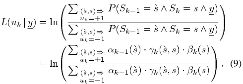
figure. From (3) and (5) we can write for the conditional LLR of , given the received sequence
(9)
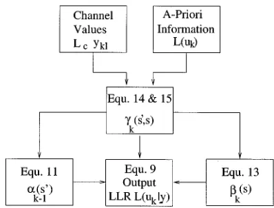
The MAP algorithm finds and for all states throughout the trellis, i.e., for , and
for all possible transitions from state to state , again for . These values are then used with (9) to give the conditional LLRs that the MAP decoder delivers. These operations are summarized in the flowchart of Fig. 4. We now describe how the values and
can be calculated.
B. The Forward Recursive Calculation of the Values
Consider first . From the definition of in (6) we can write
(10)
where in the last line we split the probability into the sum of joint probabilities over all possible previous states . Using Bayes’ rule and the assumption that the channel is memoryless again, we can proceed as follows:
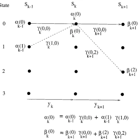
Fig. 3. Recursive calculation of (0) and (0).
Thus, once the values are known, the values can be calculated recursively. Assuming that the trellis has the initial state , the initial conditions for this recursion are
(12)
Fig. 3 shows an example of how one value, for , is calculated recursively using values of and for our example RSC code. Notice that, as we are consid-ering a binary trellis, only two previous states, and , have paths to the state . Therefore, the sum-mation in (11) is over only two terms.
C. The Backward Recursive Calculation of the Values
The values of can similarly be calculated recursively. Using a similar derivation to that for (11) it can be shown that
(13)
Thus, once the values are known, a backward recursion can be used to calculate the values of from the values of using (13). Fig. 3 again shows an example of how the
value is calculated recursively using values of
and for our example RSC code.
D. Calculation of the Values
We now consider how the transition probability values in (5) can be calculated from the received channel sequence and any a-priori information that is available. Using the definition of from (8) and the derivation from Bayes’ rule we have
(14)
where
input bit necessary to cause the transition from state
to state ;
a-priori probability of this bit;
transmitted codeword associated with this transition. Hence, the transition probability is given by the product of the a-priori probability of the input bit necessary for the transisiton, and the probability that given the codeword as-sociated with the transition was transmitted we received the channel sequence . The a-priori probability is derived in an iterative decoder from the output of the previous compo-nent decoder, and the conditional received sequence probability is given, assuming a memoryless Gaussian channel with BPSK modulation, as
(15)
where
and individual bits within the transmitted and re-ceived codewords and ;
number of these bits in each codeword; transmitted energy per bit;
noise variance;
fading amplitude (we have for nonfading AWGN channels).
E. Summary of the MAP Algorithm
From the description given above, we see that the MAP de-coding of a received sequence to give the a-posteriori LLR
can be carried out as follows. As the channel values are received, they and the a-priori LLRs (which are pro-vided in an iterative turbo decoder by the other component de-coder—see Section IV) are used to calculate according to (14) and (15). As the channel values are received, and the values are calculated, the forward recursion from (11) can be used to calculate . Once all the channel values have been received, and has been calculated for all , the backward recursion from (13) can be used to calculate the values. Finally, all the calculated
values of and are used in (9) to
calcu-late the values of . These operations are summarized in the flowchart of Fig. 4. Care must be taken to avoid numerical underflow problems in the recursive calculation of and , but such problems can be avoided by careful normal-ization of these values. Such normalnormal-ization cancels out in the ratio in (9) and so causes no change in the LLRs produced by the algorithm.
Fig. 4. Summary of the key operations in the MAP algorithm.
operations required to calculate using (9). However, much work has been done to reduce this complexity, and the Log-MAP algorithm [7], which will be described in Section V, gives the same performance as the MAP algorithm, but at a sig-nificantly reduced complexity and without the numerical prob-lems described above. In the next section we will first describe the principles behind the iterative decoding of turbo codes, and how the MAP algorithm described in this section can be used in such a scheme, before detailing the Log-MAP algorithm.
IV. ITERATIVETURBODECODINGPRINCIPLES
A. Turbo Decoding Mathematical Preliminaries
In this section, we explain the concepts of extrinsic and in-trinsic information as used by Berrou et al. [1], and highlight how the MAP algorithm described in the previous section, and other soft-in soft-out decoders, can be used in the iterative de-coding of turbo codes.
It can be shown [1] that, for a systematic code such as a RSC code, the output from the MAP decoder, given by (9), can be re-written as
(16)
where
(17)
Here, is the a-priori LLR given by (1), and is called the channel reliability measure and is given by
(18)
is the received version of the transmitted systematic bit and
(19)
Thus, we can see that the a-posteriori LLR calcu-lated with the MAP algorithm can be thought of as comprising
of three terms— and . The a-priori LLR
term comes from in the expression for the branch transition probability in (14). This probability should come from an independent source. In most cases we will have no independent or a-priori knowledge of the likely value of the bit , and so the a-priori LLR will be zero, corresponding to an a-priori probability . However, in the case of an iterative turbo decoder, each component decoder can provide the other decoder with an estimate of the a-priori LLR , as described later.
The second term in (16) is the soft output of the channel for the systematic bit , which was directly transmitted across the channel and received as . When the channel signal-to-noise (SNR) is high, the channel reliability value of (18) will be high and this systematic bit will have a large influence on the a-posteriori LLR . Conversely, when the channel is poor and is low, the soft output of the channel for the received systematic bit will have less impact on the a-posteriori LLR delivered by the MAP algorithm.
The final term in (16), , is derived, using the con-straints imposed by the code used, from the a-priori information sequence and the received channel information sequence , excluding the received systematic bit and the a-priori in-formation for the bit . Hence, it is called the extrinsic LLR for the bit . Equation (16) shows that the extrinsic infor-mation from a MAP decoder can be obtained by subtracting the a-priori information and the received systematic channel input from the soft output of the decoder. This is the reason for the subtraction paths shown in Fig. 1. Equations similar to (16) can be derived for the other component decoders which are used in iterative turbo decoding.
We summarize below what is meant by the terms a-priori, a-posteriori, and extrinsic information which are central concepts behind the iterative decoding of turbo codes use throughout this treatise.
a-priori The a-priori information about a bit is infor-mation known before decoding starts, from a source other than the received sequence or the code constraints. It is also sometimes referred to as intrinsic information to contrast with the extrinsic information described next.
extrinsic The extrinsic information about a bit is the information provided by a decoder based on the received sequence and on a-priori infor-mation excluding the received systematic bit and the a-priori information for the bit . Typically, the component decoder provides this information using the constraints imposed on the transmitted sequence by the code used. It processes the received bits and a-priori information surrounding the system-atic bit , and uses this information and the code constraints to provide information about the value of .
account all available sources of information about . It is the a-posteriori LLR, i.e., , that the MAP algorithm gives as its output.
B. Iterative Turbo Decoding
We now describe how the iterative decoding of turbo codes is carried out. Consider initially the first component decoder in the first iteration. This decoder receives the channel sequence containing the received versions of the transmitted sys-tematic bits , and the parity bits , from the first en-coder. Usually, to obtain a half rate code, half of these parity bits will have been punctured at the transmitter, and so the turbo de-coder must insert zeros in the soft channel output for these punctured bits. The first component decoder can then process the soft channel inputs and produce its estimate of the conditional LLRs of the data bits . In this notation, the subscript 11 in indicates that this is the a-posteriori LLR in the first iteration from the first component decoder. Note that in this first iteration the first component de-coder will have no a-priori information about the bits, and hence
in (14) giving will be 0.5.
Next, the second component decoder comes into operation. It receives the channel sequence containing the interleaved version of the received systematic bits, and the parity bits from the second encoder. Again the turbo-decoder will need to insert zeroes into this sequence if the parity bits generated by the encoder are punctured before transmission. However, now, in addition to the received channel sequence , the decoder can use the conditional LLR provided by the first component decoder to generate a-priori LLRs to be used by the second component decoder. Metaphorically speaking, these a-priori LLRs —which are related to bit —would be provided by an “independent conduit of in-formation, in order to have two independent channel-impaired opinions” concerning bit . This would provide a “second channel-impaired opinion” as regards to bit . In an iterative turbo decoder, the extrinsic information from the other component decoder is used as the a-priori LLRs, after being interleaved to arrange the decoded data bits in the same order as they were encoded by the second encoder. The second component decoder thus uses the received channel sequence and the a-priori LLRs (derived by interleaving the extrinsic LLRs of the first component decoder) to produce its a-posteriori LLRs . This is then the end of the first iteration.
For the second iteration the first component encoder again processes its received channel sequence , but now it also has a-priori LLRs provided by the extrinsic portion of the a-posteriori LLRs calculated by the second component encoder, and hence it can produce an improved a-posteriori LLR . The second iteration then continues with the second component decoder using the improved a-posteriori LLRs from the first encoder to derive, through (16), improved a-priori LLRs which it uses in conjunction with its received channel sequence
to calculate .
This iterative process continues, and with each iteration on average the BER of the decoded bits will fall. However, in [18, Fig. 9], the improvement in performance for each additional iteration carried out falls as the number of iterations increases. Hence, for complexity reasons usually only around six to eight iterations are carried out, as no significant im-provement in performance is obtained with a higher number of iterations.
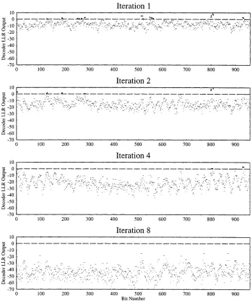
Fig. 5 shows how the a-posteriori LLRs output from the component decoders in an iterative decoder vary with the number of iterations used. The output from the second component decoder is shown after one, two, four, and eight iterations. The input sequence consisted entirely of 1 values, hence negative a-posteriori LLR values correspond to a correct hard decision, and positive values to an incorrect hard decision. The encoded bits were transmitted over an AWGN channel at a channel SNR of 1 dB, and then decoded using an iterative turbo decoder using the MAP algorithm. It can be seen that as the number of iterations used increases, the number of positive a-posteriori LLR values, and hence the BER, decreases until after eight iterations there are no incorrectly decoded values. Furthermore, as the number of iterations increases, the decoders become more certain about the value of the bits and hence the magnitudes of the LLRs gradually become larger. The erroneous decisions in the figure appear in bursts, since deviating from the error-free path trellis path typically inflicts several bit errors.
When the series of iterations finishes the output from the turbo decoder is given by the de-interleaved a-posteriori LLRs of the second component decoder, , where is the number of iterations used. The sign of these a-posteriori LLRs gives the hard decision output, i.e., whether the decoder believes that the transmitted data bit was 1 or 1, and in some ap-plications the magnitude of these LLRs, which gives the confi-dence the decoder has in its decision, may also be useful.
Fig. 5. Soft outputs from the MAP decoder in an iterative turbo decoder for a transmitted stream of all01.
to the bit . When this extrinsic LLR is used as the a-priori LLR by the other component decoder, because of the interleaving used, the bit and its neighbors will probably have been well separated. Henc, the dependence of the a-priori LLRs on the received systematic channel values which are also used by the other component decoder will have relatively little effect, and the iterative decoding provides good results.
Another justification for using the iterative arrangement described above is how well it has been found to work. In the limited experiments that have been carried out with op-timal decoding of turbo codes [21]–[23] it has been found that optimal decoding performs only a fraction of a decibel (around 0.35–0.5 dB) better than iterative decoding with the MAP algorithm. Furthermore, various turbo coding schemes have been found [23], [24], that approach the Shannonian limit, which gives the best performance theoretically available, to a similar fraction of a decibel. Therefore, it seems that, for a variety of codes, the iterative decoding of turbo codes gives an
almost optimal performance. Hence, it is this iterative decoding structure, which is almost exclusively used with turbo codes.
Having described how the MAP algorithm can be used in the iterative decoding of turbo codes, we now proceed to de-scribe other soft-in soft-out decoders, which are less complex and can be used instead of the MAP algorithm. In the forth-coming section, we first describe two related algorithms, the Max-Log-MAP [25], [26] and the Log-MAP [7], which are de-rived from the MAP algorithm, and then another, referred to as the SOVA [8], [9], [19], derived from the Viterbi algorithm.
V. MODIFICATIONS OF THEMAP ALGORITHM
A. Introduction
its complexity can be dramatically reduced without affecting its performance. Initially the Max-Log-MAP algorithm was pro-posed by Koch and Baier [25] and Erfanian et al. [26]. This technique simplified the MAP algorithm by transferring the re-cursions into the log domain and invoking an approximation to dramatically reduce the complexity. Because of this approxima-tion its performance is sub-optimal compared to that of the MAP algorithm. However, Robertson et al. [7] in 1995 proposed the Log-MAP algorithm, which corrected the approximation used in the Max-Log-MAP algorithm and hence gave a performance identical to that of the MAP algorithm, but at a fraction of its complexity. These two algorithms are described in this section.
B. Mathematical Description of the Max-Log-MAP Algorithm
The MAP algorithm calculates the a-posteriori LLRs using (9). To do this requires the following values: 1) The values, which are calculated in a forward
recursive manner using (11);
2) the values, which are calculated in a backward re-cursion using (13),; and
3) the branch transition probabilities , which are cal-culated using (14).
The Max-Log-MAP algorithm simplifies this by transferring these equations into the log arithmetic domain and then using the approximation
(20)
where means the maximum value of . Then, with and defined as follows:
(21)
(22)
and
(23)
we can rewrite (11) as
(24)
Equation (24) implies that for each path in Fig. 2 from the pre-vious stage in the trellis to the state at the present stage, the algorithm adds a branch metric term to the previous value to find a new value for that path. The new value of according to (24) is then the maximum of the values of the various paths reaching the state . This can be thought of as selecting one path as the “survivor” and discarding any other paths reaching the state. The value of should give the natural logarithm of the probability that the trellis is in state at stage , given that the received
channel sequence up to this point has been . However, be-cause of the approximation of (20) used to derive (24), only the Maximum Likelihood (ML) path through the state is considered when calculating this probability. Thus, the value of in the Max-Log-MAP algorithm actually gives the prob-ability of the most likely path through the trellis to the state , rather than the probability of any path through the trellis to state . This approximation is one of the reasons for the sub-optimal performance of the Max-Log-MAP algorithm com-pared to the MAP algorithm.
We see from (24) that in the Max-Log-MAP algorithm the forward recursion used to calculate is exactly the same as the forward recursion in the Viterbi algorithm—for each pair of merging paths the survivor is found using two additions and one comparison. Notice that for binary trellises the summation, and maximization, over all previous states in (24) will in fact be over only two states, because there will be only two previous states with paths to the present state . For all other values of we will have .
Similarly to (24) for the forward recursion used to calculate the , we can rewrite (13) as
(25)
giving the backward recursion used to calculate the
values. Again, this is equivalent to the recursion used in the Viterbi algorithm except it proceed backward rather than for-waards through the trellis.
Using (14) and (15), we can write the branch metrics in the above recursive equations for and as
(26)
where does not depend on or on the transmitted codeword and so can be considered a constant and omitted. Hence, the branch metric is equivalent to that used in the Viterbi al-gorithm, with the addition of the a-priori LLR term . Furthermore, the correlation term is weighted by the channel reliability value of (18).
Finally, from (9), we can write for the a-posteriori LLRs which the Max-Log-MAP algorithm calculates
(27)
both of these groups the transition giving the maximum value of is found, and the a-posteriori LLR is calculated based on only these two “best” transitions.
The Max-Log-MAP algorithm can be summarized as follows. Forward and backward recursions, both similar to the forward recursion used in the Viterbi algorithm, are invoked to calculate using (24) and employing (25). The branch metric is given by (26), where the constant term can be omitted. Once both the forward and backward recursions have been carried out, the a-posteriori LLRs can be calculated using (27). Thus the complexity of the Max-Log-MAP algorithm is not significantly higher than that of the Viterbi algorithm—in-stead of one recursion two are carried out, the branch metric of (26) has the additional a-priori term term added to it, and for each bit (27) must be used to give the a-posteriori LLRs. Viterbi states [27] that the complexity of the Log-MAP-Max al-gorithm is no greater than three times that of a Viterbi decoder. Unfortunately the storage requirements are much greater due to the need to store both the forward and backward recursively
calculated metrics and before the values
can be calculated. However, Viterbi also states [27], [28] that by increasing the computational load slightly, to four times that of the Viterbi algorithm, the memory requirements can be dramati-cally reduced to become essentially equal to those of the Viterbi decoder.
C. Correcting the Approximation—The Log-MAP Algorithm
The Max-Log-MAP algorithm gives a slight degradation in performance compared to the MAP algorithm due to the approx-imation of (20). When used for the iterative decoding of turbo codes, Robertson et al. [7] found this degradation to result in a drop in performance of about 0.35 dB. However, the approxima-tion of (20) can be made exact by using the Jacobian logarithm
(28)
where can be thought of as a correction term. This is then the basis of the Log-MAP algorithm proposed by Robertson et al. [7]. Similarly to the Max-Log-MAP algorithm, values for
and are calculated
using a forward and a backward recursion. However, the max-imization in (24) and (25) is complemented by the correction term in (28). This means that the exact rather than approximate values of and are calculated. The correction term need not be computed for every value of , but instead can be stored in a look-up table. Robertson et al. [7] found that such a look-up table need contain only eight values for , ranging be-tween 0 and 5. This means that the Log-MAP algorithm is only slightly more complex than the Max-Log-MAP algorithm, but it gives exactly the same performance as the MAP algorithm. Therefore, it is a very attractive algorithm to use in the compo-nent decoders of an iterative turbo decoder.
Having described two techniques based on the MAP algo-rithm, which exhibited reduced complexity, in the next section we highlight the principles of an alternative soft-in soft-out de-coder based on the Viterbi algorithm.
VI. THESOVA ALGORITHM
A. Mathematical Description of the SOVA Algorithm
In this section, we describe a variation of the Viterbi algo-rithm, referred to as the SOVA [9], [19]. This algorithm has two modifications over the classical Viterbi algorithm which allow it to be used as a component decoder for turbo codes. Firstly the path metrics used are modified to take account of a-priori information when selecting the ML path through the trellis. Sec-ondly, the algorithm is modified so that it provides a soft output in the form of the a-posteriori LLR for each decoded bit.
The first modification is easily accomplished. Consider the state sequence which gives the states along the surviving path at state at stage in the trellis. The probability that this is the correct path through the trellis is given by
(29)
As the probability of the received sequence for transitions up to and including the th transition is constant for all paths
through the trellis to stage , the probability that the path is the correct one is proportional to . Therefore, our metric should be defined so that maximizing the metric will maximize . The metric should also be easily com-putable in a recursive manner as we go from the th stage in the trellis to the th stage. If the path at the th stage has the path for its first transitions then, assuming a mem-oryless channel and using the definition of from (8), we will have
(30)
A suitable metric for the path is therefore , where
(31)
Using (26) and omitting the constant term we then have
(32)
Hence, our metric in the SOVA algorithm is updated as in the Viterbi algorithm, with the additional term included so that the a-priori information available is taken into account. Notice that this is equivalent to the forward recursion in (24) used to calculate in the Max-Log-MAP algorithm.
its metric is higher, then we can define the metric difference as
(33)
The probability that we have made the correct decision when we selected path as the survivor and discarded path , is then
correct decision at
(34)
Upon taking into account our metric definition in (31) we have
correct decision at
(35)
and the LLR that this is the correct decision is simply given by .
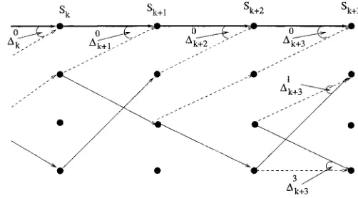
Fig. 6 shows a simplified section of the trellis of the RSC code, with the metric differences marked at various points in the trellis.
When we reach the end of the trellis and have identified the ML path through the trellis, we need to find the LLRs giving the reliability of the bit decisions along the ML path. Observations of the Viterbi algorithm have shown that all the surviving paths at a stage in the trellis will normally have come from the same path at some point before in the trellis. This point is taken to be at most transitions before , where usually is set to be five times the constraint length of the convolutional code. Therefore, the value of the bit associated with the transition from state to state on the ML path may have been different if, instead of the ML path, the Viterbi algorithm had selected one of the paths which merged with the ML path up to transitions later, i.e., up to the trellis stage . By the arguments above if the algorithm had selected any of the paths which merged with the ML path after this point the value of would not be affected, because such paths will have diverged from the ML path after the transition from to . Thus, when calculating the LLR of the bit , the soft output Viterbi algorithm (SOVA) must take account of the probability that the paths merging with the ML path from stage to stage in the trellis were incorrectly discarded. This is done by considering the values of the metric difference for all states along the ML path from trellis stage to . It is shown by Hagenauer in [29] that this LLR can be approximated by
(36)
[image:10.612.298.549.62.201.2]where is the value of the bit given by the ML path, and is the value of this bit for the path which merged with the ML path and was discarded at trellis stage . Thus the minimization in (36) is carried out only for those paths merging with the ML path which would have given a different value for the bit if they had been selected as the survivor. The paths which merge with the ML path, but would have given the same value for as the ML path, obvi-ously do not affect the reliability of the decision of .
Fig. 6. Simplified section of the trellis for ourK = 3 RSC code with SOVA decoding.
For clarification of these operations refer again to Fig. 6 showing a simplified section of the trellis for the RSC code. In this figure, as before, solid lines represent transitions taken when the input bit is a 1, and dashed lines represent transitions taken when the input bit is a 1. We assume that the all-zero path is identified as the ML path, and this path is shown as a bold line. Also shown are the paths which merge with this ML path. It can be seen from the figure that the ML path gives a value of for , but the paths merging with the ML path at trellis stages and all give a value of 1 for the bit . Hence, if we assume for simplicity that , from (36) the LLR will be given by 1 multiplied by the minimum of the metric differences and .
B. Implementation of the SOVA Algorithm
The SOVA algorithm is implemented as follows. For each state at each stage in the trellis the metric is calculated for both of the two paths merging into the state using (32). The path with the highest metric is selected as the survivor, and for this state at this stage in the trellis a pointer to the previous state along the surviving path is stored, just as in the classical Viterbi algorithm. However, in order to allow the reliability of the de-coded bits to be calculated, the information used in (36) to give is also stored. Thus the difference between the metrics of the surviving and the discarded paths is stored, to-gether with a binary vector containing bits, which indicate whether or not the discarded path would have given the same series of bits for back to as the surviving path does. This series of bits is called the update sequence in [29], and as noted by Hagenauer it is given by the result of a modulo two addition (i.e., an exclusive-or operation) between the previous decoded bits along the surviving and dis-carded paths. When the SOVA has identified the ML path, the stored update sequences and metric differences along this path are used in (36) to calculate the values of .
Let us now augment our understanding of iterative turbo de-coding by considering a specific example in the next section.
VII. TURBODECODINGEXAMPLE
In this section, we discuss an example of turbo decoding using the SOVA algorithm [9], [19] detailed in Section VI. This ex-ample serves to illustrate the details of the SOVA algorithm and the iterative decoding of turbo codes discussed in Section IV.
We consider a simple half-rate turbo code using the RSC code. The reason for using RSC codes instead of conven-tional nonsystematic, nonrecursive codes is two-fold, which we attempt to make plausible at this stage. Firstly, it would be rather wasteful in terms of both transmitted signal energy and bit rate to transmit the information and the parity bits of both compo-nent encoders twice. This would namely erode the performance benefits of turbo coding. If, however, a systematic component encoder is used, it is straightforward to puncture or obliterate one of the original systematic information bits from the trans-mitted bitstream. Furthermore, systematic codes impose less constraints on the encoded bitstream, than their nonsystematic counterparts, since in systematic encoders the original infor-mation bits are directly copied to the encoder’s output. Hence, the systematic codes exhibit a slightly better BER performance, than the nonsystematic codes, since the latter codes are over-whelmed by the plethora of channel errors and hence precip-itate more errors upon attempting to correct errors, when the channel BER is high. Since turbo codes are of most interest at high-channel BERs, systematic codes are preferred.
Secondly, the importance of the recursive nature of the RSC encoder can be made plausible as follows. For a nonrecursive convolutional code the trellis path corresponding to an input
sequence of containing a
single emerges from and merges back into the all-zero trellis path within a finite number of trellis transitions, depending on the minimum distance of the code. For recursive codes however, the input sequence would result in a eternally cycling through the encoder’s shift register stages, such that the corresponding trellis path never remerges into the all-zero path. This would result in an output sequence containing an infinite number of “ ”s. Since their associated output is quite different, the closest neighbor transmitted sequences of (the all-“ ” dataword) and above would rarely be confused with each other in the decoder in the case of recursive component codes. The path corresponding to is hence a very unlikely deviation from the all-zero path during the decoding process in the case of a recursive code, whereas it is the most likely deviation for a nonrecursive code.
[image:11.612.362.492.62.216.2]Following the above brief justification for using RSC codes the generator polynomials are expressed in octal form as 7 and 5, as shown in [18, Fig. 6]. Two such codes are combined, as shown in [18, Fig. 7], with a block interleaver to give a simple turbo code. The parity bits from both the component codes are punctured, so that alternate parity bits from the first and the second component encoder are transmitted. Thus the first, third, fifth, seventh, and ninth parity bits from the first component encoder are transmitted, and the second, fourth, sixth, and eighth
Fig. 7. State transition diagram for the(2; 1; 3) RSC component codes.
parity bits from the second component encoder are transmitted. The first component encoder is terminated using two bits chosen to take this encoder back to the all zero state. The transmitted sequence will therefore contain nine systematic and nine parity bits. Of the systematic bits, seven will be the input bits, and two will be the bits chosen to terminate the first trellis. Of the nine parity bits, five will come from the first encoder, and four from the second encoder.
The state transition diagram for the component RSC codes is shown in Fig. 7. As in all our diagrams in this section, a solid line denotes a transition resulting from a 1 input bit, and a dashed lines represents an input bit of 1. The figures within the boxes along the transition lines give the output bits associated with that transition—the first bit is the systematic bit, which is the same as the input bit, and the second is the parity bit.
For the sake of simplicity we assume that an all 1 input se-quence is used. Thus there will be seven input bits which are 1, and the encoder trellis will remain in the state. The two bits necessary to terminate the trellis will be 1 in this case and, as can be seen from Fig. 7, the resulting parity bits will also be 1. Thus, all 18 of the transmitted bits will be 1 for an all 1 input sequence. Assuming that BPSK modu-lation is used with the transmitted symbols being 1 or 1, the transmitted sequence will be a series of 18 1’s. The received channel output sequence for the example-together with the input and the parity bits detailed above are shown in Table V. Notice that approximately half the parity bits from each component en-coder are puncturedthis is represented by a dash in Table V. Also note that the received channel sequence values shown in Table V are the matched filter outputs, which were denoted by in pre-vious sections. If hard decision demodulation were used then negative values would be decoded as 1’s, and positive values as 1’s. It can be seen that from the 18 coded bits which were transmitted, all of which were 1, three would be decoded as
1 if hard decision demodulation were used.
Fig. 8. Trellis diagram for the Viterbi decoding of the received sequence shown in Table V.
1’s would be employed to terminate the trellis, and the trans-mitted sequence would consist of 18 1’s, just as for our turbo coding example. If the received sequence was as shown in Table V, then the Viterbi algorithm decoding this sequence would have the trellis diagram shown in Fig. 8. The metrics shown in this figure are given by the cross correlation of the received and ex-pected channel sequences for a given path, and the Viterbi al-gorithm maximizes this metric to find the ML path, which is shown by the bold line in Fig. 8. Notice that at each state in the trellis where two paths merge, the path with the lower metric is discarded and its metric is shown crossed out in the figure. As can be seen from Fig. 8, the Viterbi algorithm makes an incor-rect decision at stage in the trellis and selects a path other than the all zero path as the survivor. This results in three of the seven bits being decoded incorrectly as 1’s.
Having seen how Viterbi decoding of a RSC convolutional code would fail and produce three errors given the received se-quence, we now proceed to detail the operation of an iterative turbo decoder for the same channel sequence. Consider first the operation of the first component decoder in the first iteration. The component decoder uses the SOVA algorithm to decide upon not only the most likely input bits, but also the LLRs of these bits, as described in Section VI.
The metric for the SOVA algorithm is given by (32), which is repeated here for convenience
(37)
As initially we are considering the operation of the first decoder in the first iteration there is no a-priori information and hence we have for all , which corresponds to an a-priori probability of 0.5. The received sequence given in Table V was derived from the transmitted channel sequence (which has
) by adding AWGN with variance . Hence, as the fading amplitude is , from (18) we have for the channel reliability
measure .
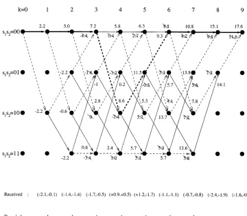
Fig. 9 shows the trellis for this first component decoder in the first iteration. Due to the puncturing of the parity bits used at the encoder, the second, fourth, sixth, and eighth parity bits have been received as zeros. The a-priori and channel values shown in Fig. 9 are given as and so that the metric values, given by (37), can be calculated by simple addition and subtraction of the values shown. As we have and , these metrics are again given by the cross correlation of the expected and received channel sequences. Notice however, that because of the puncturing used the metric values shown in Fig. 9 are not the same as those in Fig. 8. Despite this the ML path, shown by the bold line in Fig. 9, is the same as the one that was chosen by the Viterbi algorithm shown in Fig. 8, with three of the input bits being decoded as 1’s rather than 1’s.
de-Fig. 9. Trellis diagram for the SOVA decoding in the first iteration of the first decoder.
Fig. 10. Simplified trellis diagram for the SOVA decoding in the first iteration of the first decoder.
fined update sequences that indicate for which of the bits the survivor and discarded paths would have given different values, are stored by the SOVA algorithm for each node at each stage in the trellis. When the ML path has been identified, the algo-rithm uses these stored values along the ML path to find the LLR
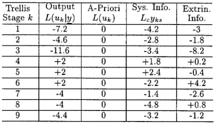
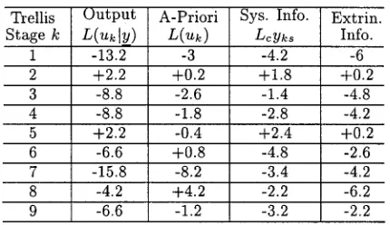
for each decoded bit. Table I shows these stored values for the example trellis shown in Figs. 9 and 10. The calculation of the decoded LLRs shown in this table is detailed below.
[image:13.612.122.472.299.603.2]TABLE I
SOVA OUTPUT FOR THEFIRSTITERATION OF THEFIRSTDECODER
be seen from Figs. 9 and 10, there are no paths merging with the ML path at these stages. For all subsequent stages there is a merging path, and values of the metric differences and update sequences are stored. For the update sequence a “1” indicates that the ML and the discarded merging path would have given different values for a particular bit. At stage in the trellis we have taken the Most Significant Bit (MSB), on the left-hand side, to represent , the next bit to represent , etc. until the Least Significant Bit (LSB), which represents . For the RSC code any two paths merging at trellis stage give different values for the bit , and so the MSB in the update sequences in Table I is always 1. Notice furthermore that although in the example the update sequences are all of different lengths, this is only because of the very short frame length we have used. More generally, as explained in Section VI, all the stored update sequences will be bits long, where is usually set to be five times the constraint length of the convolutional code.
We now explain how the SOVA algorithm can use the stored update sequences and metric differences along the ML path to calculate the LLRs for the decoded bits. Equation (36) shows that the decoded a-posteriori LLR for a bit is given by the minimum metric difference of merging paths along the ML path. This minimum is taken only over the metric
differ-ences for stages where the value
of the bit given by the path merging with the ML path at stage is different from the value given for this bit by the ML path. Whether or not the condition is met is deter-mined using the stored update sequences. Denoting the update sequence stored at stage along the ML path as , for each bit the SOVA algorithm examines the MSB of , the second MSB of , etc. up to the th bit (which will be the LSB) of . For our example this examination of the update sequences is limited because of our short frame length, but the same prin-ciples are used. Taking the fourth bit as an example, to deter-mine the decoded LLR for this bit the algorithm ex-amines the MSB of in row four of Table I, the second MSB of in row five, etc. up to the sixth MSB of in row nine. It can be seen, from the corresponding rows in Table I, that only the paths merging at stages and of the trellis give values different from the ML path for the bit . Hence, the decoded LLR from the SOVA algorithm for this bit is calculated using (36) as the value of the bit given by the ML path times the minimum of the metric differences stored at Stages 4 and 6 of the trellis (7.2 and 2), yeilding .
The remaining decoded LLR values in Table I are computed following a similar procedure. However, it is worth noting explicitly that the low value (2) of the metric difference for the merging path at Stage 6 in the trellis, which is where the incorrect path is chosen as the survivor, gives the LLR for the bits where this path and the ML path give different values. Hence, the LLRs for the three incorrectly decoded bits, i.e., and , have the lowest magnitudes of any of the decoded bits.
We now move on to describing the operation of the second component decoder in the first iteration. This decoder uses the extrinsic information from the first decoder as a-priori information to assist its operation, and therefore should be able to provide a better estimate of the encoded sequence than the first decoder was. Equation (16) from Section IV give the extrinisic information from a component decoder as the soft output from the decoder with the a-priori information (if any was available) and the received systematic channel information subtracted. This is equivalent to [18, eq. (13)]. Table II shows the extrinsic information calculated from (16) from the first decoder, which is then interleaved by a block interleaver and used as the a-priori information for the second component decoder. The second component decoder also uses the interleaved received systematic channel values, and the received parity bits from the second encoder which were not punctured (i.e., the second, fourth, sixth, and eighth bits).
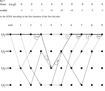
Fig. 11 shows the trellis for the SOVA decoding of the second decoder in the first iteration. The extrinsic information values from Table II are shown after being interleavered and divided by two as . Also shown is the channel information used by this decoder. Notice that as the trellis is not terminated for the second component encoder, paths termi-nating in all four possible states of the trellis are considered at the decoder. However, the metric for the state is the maximum of the four final metrics, and hence this all zero state is used as the final state of the trellis.
The ML path chosen by the second component decoder is shown by a bold line in Fig. 11, together with the LLR values output by the decoder. These are calculated, using update se-quences and minumum metric differences, in the same way as was explained for the first decoder using Fig. 10 and Table I. It can be seen that the decoder makes an incorrect decision at stage in the trellis and selects a path other than the all zero path as the survivor. However, the incorrectly chosen path gives decoded bits of 1 for only two transitions, and hence only two, rather than three, decoding errors are made. Further-more, the difference in the metrics between the correct and the chosen path at trellis stage is only 2.2, and so the mag-nitude of the decoded LLRs for the two incorrectly decoded bits, and , is only 2.2. This is significantly lower than the magnitudes of the LLRs for the other bits, and indicates that the algorithm is less certain about these two bits being 1 than it is about the other bits being 1.
Fig. 11. Trellis diagram for the SOVA decoding in the first iteration of the second decoder.
TABLE II
CALCULATION OF THEEXTRINSICINFORMATION FROM THEFIRSTDECODER IN THEFIRSTITERATION
and used as the output from the turbo decoder. This de-inter-leaving would result in an output sequence which gave negative LLRs for all the decoded bits except and , which would be incorrectly decoded as 1’s as their LLRs are both 2.2. Thus, even after only one iteration, the turbo decoder has decoded the received sequence with one less error than the convolutional de-coder did. However, generally better results are achieved with more iterations, and so we now progress to describe the opera-tion of the turbo decoder in the second iteraopera-tion.
In the second, and all subsequent, iterations the first compo-nent decoder is able to use the extrinsic information from the second decoder in the previous iteration as a-priori tion. Table III shows the calculation of this extrinsic informa-tion using (16) from the second decoder in the first iterainforma-tion. It can be seen that it gives negative LLRs for all the bits except and , and for these two bits the LLRs are close to zero. This extrinsic information is then de-interleaved and used as the
a-priori information for the first decoder in the next (second) it-eration. The trellis for this decoder is shown in Fig. 12. It can be seen that this decoder uses the same channel information as it did in the first iteration. However now, in contrast to Fig. 9, it also has a-priori information, to assist it in finding the correct path through the trellis. The selected ML path is again shown by a bold line, and it can be seen that now the correct all zero path is chosen. The second iteration is then completed by finding the extrinsic information from the first decoder, interleaving it and using it as a-priori information for the second decoder. It can be shown that this decoder will also now select the all zero path as the ML path, and hence the output from the turbo decoder after the seond iteration will be the correct all 1 sequence. This concludes our example of the operation of an iterative turbo de-coder using the SOVA algorithm, leading on to a comparison of the component decoder algorithms.
VIII. COMPARISON OF THECOMPONENT DECODER ALGORITHMS
In this article, we have described in detail the iterative struc-ture and the component decoders used to decode turbo codes. A numerical example illustrating this decoding was given in the previous section. We now conclude by summarizing the operation of the algorithms which can be used as component decoders, highlighting the similarities and differences between these algorithms, and noting their relative complexities and per-formances.
Fig. 12. Trellis diagram for the SOVA decoding in the second iteration of the first decoder.
TABLE III
CALCULATION OF THEEXTRINSICINFORMATION FROM THESECONDDECODER IN THEFIRSTITERATION
1, and similarly for every transition that could occur if the input bit was 1. As these transitions are mutually exclusive, the probability of any one of them occurring is simply the sum of their individual probabilities, and hence the LLR for a bit is given by the ratio of two sums of probabilities, as in (3).
Due to the Markov nature of the trellis and the assumption that the output from the trellis is observed in memoryless noise, the individual probabilities of the transitions in (3) can be expressed as the product of three terms— and , as in (5). The terms can be calculated from the a-priori prob-abilities for the decoded bits, and the received channel informa-tion, as in (14) and (15). Then the and terms can be calculated recursively as in . (11) and (13). The MAP algorithm is optimal for the decoding of turbo codes, but is extremely com-plex. Furthermore, because of the multiplications used in the re-cursive calculation of the and terms it often suf-fers from numerical problems in practice. The Log-MAP
algo-rithm is theoretically identical to the MAP algoalgo-rithm, but trans-fers its operations to the log domain. Thus multiplications are replaced with additions, and so the numerical problems of the MAP algorithm are avoided and its complexity is dramatically reduced.
The Max-Log-MAP algorithm further reduces the com-plexity of the Log-MAP algorithm using the maximization approximation given in (20). This has two effects on the operation of the algorithm compared to that of the Log-MAP algorithm. Firstly, as can be seen by examining (27), it means that only two transitions are considered when finding the LLR
for each bit —the best transition from
to that would give and the best that would give . Similarly in the recursive calculations of the
and terms of (24)
and (25) the approximation means that only one transition, the most likely one, is considered when calculating from
the terms and from the terms. This
means that although should give the logarithm of the probability that the trellis reaches state along any path from the initial state , in fact it gives the logarithm of the probability of only the most likely path to state . Similarly should give the logarithm of the probability of the received sequence given only that the trellis is in state at stage . However, the maximization in (25) used in the recursive calculation of the terms means that only the most likely path from state to the end of the trellis is considered, and not all paths.
Hence, the Max-Log-MAP algorithm finds the LLR
that would give and the best path that would give are compared. One of these “best paths” will al-ways be the ML path, and so will not change from one stage to the next, whereas the other may change. In contrast the MAP and the Log-MAP algorithms consider every path in the calcu-lation of the LLR for each bit. All that changes from one stage to the next is the division of paths into those that give
and those that give . Thus the Max-Log-MAP algo-rithm gives a degraded performance compared to the MAP and Log-MAP algorithms.
In the SOVA algorithm the ML path is found by maximizing the metric given in (32). The recursion used to find this metric is identical to that used to find the terms in (24) in the Max-Log-MAP algorithm. Once the ML path has been found, the hard decision for a given bit is determined by which tran-sition the ML path took between trellis stages and . The LLR for this bit is determined by examining the paths which merge with the ML path that would have given a different hard decision for the bit . The LLR is taken to be the minimum metric difference for these merging paths which would have given a different hard decision for the bit . Using the notation associated with the Max-Log-MAP algorithm, once a path merges with the ML path, it will have the same value of as the ML path. Hence, as the metric in the SOVA is identical to the values in the Max-Log-MAP, taking the difference between the metrics of the two merging paths in the SOVA algorithm is equivalent to taking the difference
between two values of in the
Max-Log-MAP algorithm, as in (27). The only difference is that in the Max-Log-MAP algorithm one path will be the ML path, and the other will be the most likely path that gives a different hard decision for . In the SOVA algorithm again one path will be the ML path, but the other may not be the most likely path that gives a different hard decision for . Instead, it will be the most likely path that gives a different hard decision for and survives to merge with the ML path. Other, more likely paths, which give a different hard decision for the bit to the ML path may have been discarded before they merge with the ML path. Thus the SOVA algorithm gives a degraded performance compared to the Max-Log-MAP algorithm. However, as pointed out in [7] by Robertson et al. the SOVA and Max-Log-MAP al-gorithms will always give the same hard decisions, as in both algorithms these hard decisions are determined by the ML path, which is calculated using the same metric in both algorithms.
A comparison of the complexities of the Log-MAP, the Max-Log-MAP, and the SOVA algorithms is given in [7]. The relative complexity of the algorithms depends on the constraint length of the convolutional codes used, but it is shown that the Max-Log-MAP algorithm is about twice as complex as the SOVA algorithm. The Log-MAP algorithm is slightly more complex than the Max-Log-MAP algorithm due to the look-ups required to find the correction factors . The performance of the algorithms when used in the iterative decoding of turbo codes falls in the same order as their complexities, with the best performance given by the Log-MAP algorithm, then the Max-Log-MAP algorithm, and the worst performance given by the SOVA algorithm. In the next section we study the effect of the various parameters on the codec performance.
TABLE IV
STANDARDTURBOENCODER ANDDECODERPARAMETERSUSED
TABLE V
INPUT ANDTRANSMITTEDBITS FORTURBODECODINGEXAMPLE
IX. THEEFFECT OFVARIOUSCODECPARAMETERS
In this section we present simulation results for turbo codes using Binary Phase Shift Keying (BPSK) over Additive White Gaussian Noise (AWGN) channels. We show that there are many parameters, some of which are interlinked, which affect the performance of turbo codes. Some of these parameters are:
• The component decoding algorithm used. • The number of decoding iterations used. • The frame-length or latency of the input data. • The specific design of the interleaver used.
• The generator polynomials and constraint lengths of the component codes.
Fig. 13. Turbo coding BER performance using different numbers of iterations of the MAP algorithm. other parameters as in Table IV.
leading to a one-third rate code. At the decoder two component, soft-in soft-out, decoders are used in parallel in the structure shown in Fig. 1. In most of our simulations we use the Log-MAP decoder, but the effect of using other component decoders is in-vestigated in Section IX-C. Usually 8 iterations of the compo-nent decoders are used, but in the next section we consider the effect of the number of iterations.
A. The Effect of the Number of Iterations Used
Fig. 13 shows the performance of a turbo decoder using the MAP algorithm versus the number of decoding iterations which were used. For comparison, the uncoded BER and the BER ob-tained using convolutional coding with a standard non-recursive convolutional code, are also shown. Like the compo-nent codes in the turbo encoder, the convolutional encoder uses the optimum octal generator polynomials of 7 and 5. It can be seen that the performance of the turbo code after one iteration is roughly similar to that of the convolutional code at low SNRs, but improves more rapidly than that of the convolutional coding as the SNR is increased. As the number of iterations used by the turbo decoder increases, the turbo decoder performs signif-icantly better. However, after eight iterations there is little im-provement achieved by using further iterations. For example, it can be seen from Fig. 13 that using 16 iterations rather than eight gives an improvement of only about 0.1 dB. Similar results are obtained when using the SOVA algorithm—again there is little improvement in the BER performance of the decoder from using more than eight iterations. Hence, for complexity reasons usu-ally only about eight iterations are used, and so, unless otherwise stated, in our future simulations we have used eight iterations. In the next section, we consider the effect of puncturing.
B. The Effect of Puncturing
[image:18.612.307.549.292.485.2]Again, in a turbo encoder two or more component encoders are used to generate parity information from an input data se-quence. We have used two RSC component encoders, and this is the arrangement most commonly used for turbo codes with rates below two-thirds. Typically, in order to give a half-rate code,
Fig. 14. BER performance comparison between one-third and half-rate turbo codes using parameters of Table IV.
Fig. 15. BER performance comparison between different component decoders for a random interleaver withL = 1000. Other parameters as in Table IV.
half the parity bits from each component encoder are punctured. This was the arrangement used in their original paper by Berrou et al. on turbo codes [1]. However, it is of course possible to omit the puncturing and transmit all the parity information from both component encoders, which gives a one-third rate code. The performance of such a code, compared to the corresponding half-rate code, is shown in Fig. 14. In this figure, the encoders use the same parameters as were described above for Fig. 13. It can be seen that transmitting all the parity information gives a gain of about 0.6 dB, in terms of , at a BER of 10 . This corresponds to a gain of about 2.4 dB in terms of channel SNR. Very similar gains are seen for turbo codes with different frame-lengths. Let us now consider the performance of the var-ious soft-in soft-out component decoding algorithms.
C. The Effect of the Component Decoding Algorithm Used
Fig. 16. BER performance comparison between different component decoders for aL = 169; 13 2 13, block interleaver. Other parameters as in Table IV.
Fig. 17. BER performance comparison between different component decoders for a random interleaver withL = 1000 Using a 1=3 rate code. Other parameters as in Table IV.
10 this degradation is about 0.1 dB for the Max Log MAP algorithm, and about 0.6 dB for the SOVA algorithm.
Fig. 16 compares the Log MAP, Max Log MAP and SOVA algorithms for a turbo decoder with a frame-length of only 169 b, rather than 1000 b as was used for Fig. 15. It can be seen that although all three decoders give a worse BER performance than those shown in Fig. 15, the differences in the performances between the decoders are very similar to those shown in Fig. 15. Similarly, Fig. 17 compares these three decoding algorithms for a one-third rate code, and again the degradations relative to a decoder using the Log-MAP algorithm are about 0.1 dB for the Max-Log-MAP algorithm, and about 0.6 dB for the SOVA algorithm.
D. The Effect of the Frame-Length of the Code
[image:19.612.307.549.64.253.2]In the original paper on turbo coding by Berrou et al. [1], and many of the subsequent papers, impressive results have been presented for coding with very large frame lengths. Dolinar et al.
Fig. 18. Effect of frame-length on the BER performance of turbo coding. All Interleavers exceptL = 169 block interleaver use random separated interleavers [31]. Other parameters as in Table IV.
analyzed the associated theoretical performance limits as a func-tion of the coded frame length in [32]. However, for many appli-cations, such as speech transmission systems, the large delays inherent in using high frame-lengths are unacceptable. There-fore, an important area of turbo coding research is achieving as impressive results with short frame-lengths as have been demon-strated for long frame-length systems. Fig. 18 shows how dra-matically the performance of turbo codes depends on the frame-length used in the encoder. The 169-bit code would be suitable for use in a speech transmission systems at approximately 8 kb/s with a 20-ms frame-length [33], while the 1000–bit code would be suitable for video transmission. The larger frame-length tems would be useful in data or nonreal time transmission sys-tems. It can be seen from Fig. 18 that the performance of turbo codes is very impressive for systems with long frame lengths. However, even for a short frame-length system, using 169 b per frame, it can be seen that turbo codes give good results, com-parable to or better than a constraint length convolu-tional code. The use of the convolutional code as a bench-marker is justified below.
Fig. 15 shows a comparison between turbo decoders using the parameters described above. In this figure the “Log MAP (exact)” curve refers to a decoder which calculates the correc-tion term in (28) of Section 5 exactly, i.e., using
(38)
rather than using a look-up table as described in [7]. The Log MAP curve refers to a decoder which does use a look-up table with eight values of stored, and hence introduces an ap-proximation to the calculation of the LLRs. It can be seen that, as expected, the MAP and the Log-MAP (exact) algorithms give identical performances. Furthermore, as Robertson found [7], the look-up procedure for the values of the correction terms introduces no degradation to the performance of the de-coder.
[image:19.612.44.284.298.481.2]