Nonlinear Processes
in Geophysics
c
European Geosciences Union 2003
Sequential parameter estimation for stochastic systems
G. A. Kivman
Alfred Wegener Institute for Polar and Marine Research, Bremerhaven, Germany Received: 24 August 2001 – Revised: 7 November 2002 – Accepted: 19 December 2002
Abstract. The quality of the prediction of dynamical sys-tem evolution is determined by the accuracy to which ini-tial conditions and forcing are known. Availability of fu-ture observations permits reducing the effects of errors in assessment the external model parameters by means of a fil-tering algorithm. Usually, uncertainties in specifying inter-nal model parameters describing the inner system dynamics are neglected. Since they are characterized by strongly non-Gaussian distributions (parameters are positive, as a rule), traditional Kalman filtering schemes are badly suited to re-ducing the contribution of this type of uncertainties to the forecast errors. An extension of the Sequential Importance Resampling filter (SIR) is proposed to this aim. The filter is verified against the Ensemble Kalman filter (EnKF) in appli-cation to the stochastic Lorenz system. It is shown that the SIR is capable of estimating the system parameters and to predict the evolution of the system with a remarkably better accuracy than the EnKF. This highlights a severe drawback of any Kalman filtering scheme: due to utilizing only first two statistical moments in the analysis step it is unable to deal with probability density functions badly approximated by the normal distribution.
1 Introduction
Our ability to predict the state of the atmosphere and the ocean highly depends on the accuracy to which initial condi-tions and forcing funccondi-tions are known. Various data assim-ilation techniques have been developed to constrain models with observations in order to reduce the influence of uncer-tainties in these external model parameters on the forecast skill. In parallel with the forecast errors of this type, there are those caused by uncertainties in internal model param-eters describing the inner system dynamics (such as mix-ing and diffusivity coefficients, etc.). The so-called adjoint Correspondence to: G. A. Kivman
method borrowed from the engineering optimal control lit-erature provides a tool to tune the model to available data by adjusting those model parameters. However, this method involves an assumption that the model structure is perfect which is too restrictive for oceanographic and meteorological applications. Accounting for model errors in the parameter estimation problem dramatically increases the dimension of the control space and is affordable only for low dimensional models (ten Brummelhuis et al., 1993; Eknes and Evensen, 1997; Gong et al., 1998).
Commonly, the physical model is calibrated initially to chose some “optimal” values of the external parameters. Then a scheme of the Kalman filtering is applied for cor-recting the prediction with available data. At this stage, the model parameters are assumed to be known precisely. How-ever, neglecting uncertainties of this kind leads to overesti-mating the forecast skill. As a result, the data make a lesser contribution to the analyzed system state and the true trajec-tory of the system can be quickly lost.
A question arises of whether it is possible to embed param-eter estimation into this scheme and to optimize the internal model parametersmsequentially together with filtering the system state. Though the model parameters are not dynami-cal variables, we can easily augment the original dynamidynami-cal system
dx
dt =M(t,m,x) , (1)
by the equation
dm
dt =0. (2)
provides a very sensitive test for evaluating of how a filtering scheme deals with nonlinearity and with distributions badly approximated by the normal one.
The aim of this paper is twofold. The first objective is to demonstrate that sequential tuning of the internal param-eters is allowable by means of Monte Carlo methods with no additional computational cost. The other goal is to show that accounting for the whole error statistics leads to notably better forecast. Particle filters provide a tool for that. They are introduced in Sect. 2. Section 3 contains an example of filtering the Lorenz system with the well-known Ensemble Kalman filter (EnKF) and with the so-called Sequential Im-portance Resampling filter (SIR). An extension of the SIR to sequentially optimize the model parameters and compari-son of the SIR with an analogous extension of the EnKF is presented in Sect. 4. In previous studies, to the best of the author’s knowledge the particle filters were tested in applica-tion to estimating unknown parameters of linear dynamical systems only (Liu and West, 2001 and references therein). Section 5 contains discussion and conclusions.
2 Particle filters
It is well known, that the classical Kalman filter (KF) is op-timal in the sense of minimizing the variance only for lin-ear systems and the Gaussian statistics. A linlin-earization of the error covariance evolution used in the Extended Kalman filter (EKF) (Jazwinski, 1973) often turns out to be inade-quate. Unbounded growth of the computed error variances due to neglecting nonlinear saturation effects causes the up-date procedure to become unstable (Evensen, 1992). Miller et al. (1994, 1999) showed poor performance of the EKF in application to the Lorenz system when the data are too sparse or too inaccurate.
To go around the closure problem for the error statis-tics propagation, Evensen (1994) proposed the Ensemble Kalman filter (EnKF). The heart of the method is Monte Carlo integration of the Fokker-Planck-Kolmogorov (FPK) equation governing the evolution of the probability density function (PDF) that describes the forecast error statistics. In the analysis step, each ensemble member is updated accord-ing to the traditional scheme of the KF with the use of the forecast covariance matrix derived from the ensemble statis-tics. Then, if the data are randomly perturbed, the updated ensemble is shown to have the proper mean and covariance matrix (Burgers et al., 1998).
However, two potential problems for the EnKF are worth to mention. First, though the EnKF uses the full non-linear dynamics to propagate the forecast error statistics, it mim-ics the traditional KF in the analysis step and uses only the Gaussian part of the prior PDF. Bennett (1992) pointed out that “one thing is certain: least-squares estimation is very in-efficient for highly intermittent processes, having probability distributions not well characterized by means and variances”. Second, the updated ensemble preserves only two first mo-ments of the posterior. Consequently, the initial condition
for the further integration of the FPK does not coincide with the posterior PDF. In the case of a small system noise when the “diffusion” of probabilities is small compared with the “advection”, the system does not forget its initial state for a long time and the ensemble becomes non-representative for the forecast error statistics after few analysis steps.
Particle filters provide a tool to solve these problems. As the EnKF, they rely on Monte Carlo integration of the FPK equation. However, instead of updating ensemble members in the analysis step they update their probabilities accord-ing to the fitness to observations. Consequently, they do not involve any model reinitialization that usually injects imbal-ance in the model state and leads to a shock in the system evolution. Another advantage of these filters is that they make use of the full statistics of the forecast and data errors and thus are truly variance minimizing methods.
The basic algorithm of the particle filtering consists of the following steps:
1. An initial ensemblexn, n=1, . . . , Nis drawn from a
prior distributionρ(x).
2. Each ensemble memberxnevolves according to the
dy-namical equations.
3. Att = tk when the datadk become available, weights wn(tk)expressing “fitness” of ensemble members to the
data are computed
wn(tk)=wn(tk−1)ρ(dk|xn(tk)) (3)
and normalized so that
N
X
n=1
wn(tk)=1.
Here ρ(dk|xn(tk)) expresses the conditional PDF for
the data dk to be observed when the system state is
xn(tk)or, in other words, describes the statistics of the
data errors.
4. The final prediction is calculated as the weighted en-semble mean.
This scheme was called as the direct ensemble method in van Leeuwen and Evensen (1996). They found that the vast majority of the ensemble members got negligible weights af-ter few analysis steps and thus only a tiny fraction of the ensemble contributes to the mean. In this case, to obtain a reasonable approximation of the posterior PDF one needed to use an ensemble of about 104members. This drawback of the method is explained by a Kong-Liu-Wong theorem (Kong et al., 1994) which states that the unconditional variance of the importance weightswn, i.e. with observations treated as
random variables, increases in time. Thus, the algorithm be-comes more and more unstable.
(SIR) proposed by Rubin (1988) and applied to filtering the dynamical systems in Gordon et al. (1993). The basic idea of the method is that there is no need in computing further evolution of ensemble members having bad fitness to the data. It is achieved by generating a new ensemble of equally probable members at each analysis step by means of sam-pling from the old ensemble with replacement. Probabilities for the members to be sampled at t = tk are assigned to
their normalized weightswn(tk)calculated by Eq. (3) with wn(tk−1) = 1. Smith and Gelfand (1992) have proven that
a discrete approximation tends to the posterior PDF when the sample size tends to infinity. This is just opposite to the EnKF which does not produce an approximation to the pos-terior PDF and preserves only the mean and the covariance.
3 Filtering the Lorenz system
To compare the EnKF and the SIR filter, an identical twin experiment with the Lorenz system
dx
dt =γ (y−x) , dy
dt =rx−y−xz , (4) dz
dt =xy−βz ,
with commonly used parametersγ =10, r =28,andβ = 8/3 was performed. Each of Eqs. (4) were perturbed with white noise stochastic forcing having variances 2., 12.13 and 12.13 correspondingly. The reference solution fort ∈ [0,20] was computed starting from an initial condition obtained by adding a noiseN (0,
√
2)to the first guess
(x0, y0, z0)=(1.508870,−1.531271,25.46091) .
The observations for thex−andz−components were gen-erated at eachδt = 1 by adding theN (0,
√
2)noise to the reference solution.
The experiment design is almost identical to that of Evensen and van Leeuwen (2000). The major differences are the distance between observations which was made twice larger and that only 2 components of the model state were observable. Observability of the whole system state is the case standing far away from that we deal with in meteoro-logical and oceanographic applications. For the same reason of making the system less constrained by the data the data frequency was lowered. In addition, for more pictorial pre-sentation of results, the assimilation period was chosen to be twice shorter than that in Evensen and van Leeuwen (2000). Table 1 summarizes results of experiments made with use of the SIR and EnKF for 250 and 1000 ensemble members. As it is seen, performance of the filters improves with in-creasing the ensemble size. However, this improvement is less than 20% with four-fold increasing the ensemble size and is mostly achieved due to better representation of system oscillations near the attractor withint ∈ [7.5,11.5](compare Fig. 1 and Fig. 2). This reflects the very slow convergence of
Table 1. RMS deviation of the filtered solutions with the fixed
model parameters from the true trajectory
Filter EnKF SIR EnKF SIR
Ensemble size 250 250 1000 1000
x 7.4 6.5 6.5 5.8
y 8.9 8.1 8.4 7.3
z 8.0 7.8 7.1 6.6
Monte Carlo methods which is of the order of O(N−1/2), whereN is the amount of the ensemble members. Another important point worth to be mention is that the SIR for the smaller ensemble is almost as effective as the EnKF for the larger ensemble.
The main problem of the SIR with 250 ensemble mem-bers is its inability to capture the true trajectory withint ∈ [7.5,11.5]. The reason for this failure is bad scores of all ensemble members and consequently poor representation of the forecast error statistics. This problem for the SIR is re-covered by enlarging the ensemble. One can notice that the EnKF with the smaller ensemble does a better job within this interval. Seemingly, it is a general point. If all ensemble members deviate much from the observations, the EnKF up-dates the ensemble trajectories and improves their fit to the data, while the SIR changes the ensemble probabilities and do not do anything with fitness of the ensemble members.
The filters for the both ensemble sizes lose the true tra-jectory att = 3 when they assimilate a bad data on thex
component coming just after the transition point. Before the analysis step, both filters predict a transition, but the data wrongly tells about the absence of the transition point. The filters accept this information and delay the transition for a while. Then the EnKF predicts the next data att =4 much better than the SIR. However, it propagates the information provided by the data to the unobservedy-component much worse. As a result, the SIR solution fort ∈ [4,5]is almost identical to the true trajectory, while the EnKF catches it only att =5. This situation is a stable feature which do not de-pend on the ensemble size.
There are two more examples of inadequate transmission of the information provided by the data onxandzto the un-observedy. Let us consider the analysis step att =19 for the smaller ensemble. Both filters lost the system trajectory at aboutt=18.5. With the analysis step, they recover the ob-served components of the solution. However, the SIR makes a better inference abouty and is capable to follow the sys-tem trajectory further while the EnKF loses it immediately after the analysis step. The same situation occurs att = 7 for the larger ensemble. Inspite large deviations between the forecast and the data, the SIR places the analysis just at the system trajectory. The EnKF updates only the observed com-ponents in a proper manner while they-component is pulled even in a wrong direction.
0 5 10 15 20 −20
−10 0 10 20
X
0 5 10 15 20
−20 0 20
Y
0 5 10 15 20
0 20 40 60
X
Fig. 1. Filtered solutions for 250 ensemble members with the fixed
model parameters: the SIR – red, the EnKF – green. The blue curve is the true trajectory, circles are observations.
unobserved part of the system state always wrongly when it faces large data misfits. For example, the analysis att =12 was made by the EnKF very precisely. However, keeping in mind that the EnKF does not make use of the whole er-ror statistics one can conclude that the filter has problems in transferring the information from the data to the unobserved part of the system and they cannot be resolved with enlarging the ensemble size.
An interesting point is the reaction of the filters on chang-ing observability of the system. To investigate this issue, a series of experiments with different data errors and distances between observations was performed. First and foremost, the SIR outperforms the EnKF for the larger ensemble in any case. Seemingly, 1000 species are enough to sample properly the system phase space and, when this is the case, employing the whole error statistics is superior to using only the Gaus-sian part. However, the situation changes for the smaller en-semble. Increasing observability of the system (reducing the distance between observations and data errors) has a
signifi-0 5 10 15 20
−20 −10 0 10 20
X
0 5 10 15 20
−20 0 20
Y
0 5 10 15 20
0 20 40 60
X
Fig. 2. The same as Fig. 1 for 1000 ensemble members.
cant positive impact on the performance of the EnKF while it surprisingly degrades that of the SIR. For example, doubling the data density with keeping the data error variance fixed results in better performance of the EnKF compared to the SIR. Assimilating less accurate data of the error variance of
σ =3 √
2 recovers better performance of the SIR.
To explain this behavior one should keep in mind the fol-lowing. When the data errors are distributed according to the Gaussian statistics as in the particular example consid-ered here, the analysis step pushes the forecast error statis-tics towards the normal distribution. The better are the data and the more components of the system state are observable the higher is this effect. Further, we start initially from the Gaussian PDF. Consequently, reducing the distance between observations and the data errors prevent the forecast error statistics from moving far away from the normal distribution. Thus, one can expect higher skills of the Kalman filter in this case.
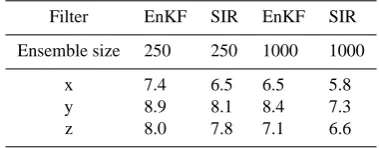
sys-Table 2. RMS deviation of the filtered solutions with the adjusted
model parameters from the true trajectory
Filter EnKF SIR EnKF SIR
Ensemble size 250 250 1000 1000
x 9.2 7.1 9.7 5.6
y 10.6 8.2 11.0 7.1
z 14.2 7.7 14.7 6.6
tem phase space in this case that becomes more pronounced with increasing the data density and data quality. In addition, resampling artificially decreases the ensemble spread. This may cause the deterioration of the filter performance with extending the assimilation period. Indeed, whenδt = 0.5 andσ =
√
2, the SIR still works better than the EnKF for
t ∈ [0,10]but then its skills drastically fall down due to the ensemble collapse.
4 Sequential combined parameter- and state estimation with the SIR filter
Extension of the SIR and the EnKF for the system (1), (2) is straightforward. To examine their potentialities, the ex-periment described in Sect. 3 was repeated with the initial ensemble in the parameter space drawn from the uniform dis-tribution forγ ∈ [0,30.]andr ∈ [0,44.8]. While evolving each particular ensemble member,γ andrwere kept equal to their initial values and the data choose whether these values are close to the truth (and the ensemble member survives at the analysis step) or not (the ensemble member dies).
Estimating static parameters is a tough problem for the SIR. If the major part of the ensemble has bad fitness to the data due to undersampling or wrong prior statistics, only few members will be resampled while the absence of the noise in the parameter space will not allow the ensemble to regain the spread. As was mentioned in Sect. 3, it may cause difficul-ties for the SIR. A possible solution is to add some noise to the resampled parameters to stabilize the filter analogous to introducing the forgeting factor (Pham, 2001). However, this procedure involves an arbitrary regularization parameter (the noise level) to be tuned that complicates the comparison of two filters.
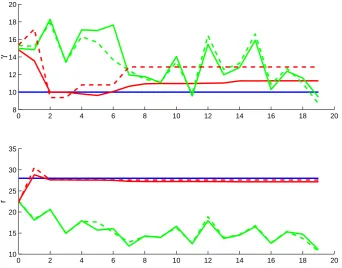
One can easily verify that the system trajectory is more sensitive to the choice ofr. Thus, it is not a surprise that the SIR catches the value ofrafter the first analysis step (Fig. 3). The next analysis step produces a very good estimate forr. However, it is impaired with time until the filter collapses in the parameter space. Since the trajectory of the system is tolerant to variations ofγ, the quality of the filtered solution (see Table 2) which is of our primary interest still remains almost identical to that presented in Sect. 3.
It is not the case for the EnKF. In the parameter estimation problem, the EnKF has to deal with the PDFs badly approx-imated by the Gaussian distribution. Such a modification in
the problem formulation completely corrupts the filter per-formance. The solution produced by the EnKF has very little common with the true trajectory and its quality does not de-pend on the ensemble size (see Table 2).
The failure of the EnKF is caused by its incapability to re-cover the true values of the model parameters (see Fig. 3). The evolution of estimates forγ resembles a random walk over the parameter subspace. As we can expect and it was the case for the SIR, this parameter is derived from the data with a lower accuracy compared to that forr. It is astonishing that the EnKF does even a much worse job when estimating the more crucial parameterr. After removing fluctuations from the corresponding curve presented in Fig. 3, one can easily see a pronounced tendency of pushing the estimates of
rin the opposite direction with respect to the true value. It is worth noting that the parameter estimates obtained with the EnKF for the both ensembles are indistinguishable. These point out that the EnKF is completely unable to deal with the PDFs defined over constrained sets. An additional evidence for this conclusion is that the EnKF was permanently trying to produce negative analyzed parameter values for some en-semble members and the condition of non-negativeness had to be imposed by force.
In the experiment described above the true value forβwas specified. Results remain similar to those presented when the truth deviates from the prescribed value within the 10% error. Otherwise, the SIR was unable to locaterandγ properly and to follow the system trajectory. This points out to necessity of a preliminary sensitivity analysis to detect the most crucial model parameters to be adjusted before running the filter.
5 Discussion and conclusions
Data assimilation for high-dimensional nonlinear ocean and atmospheric models is a challenging task. On the one side, high-dimensionality forces us to use simplified representa-tion of the error statistics and thus to neglect some sources of uncertainties. Developing approaches for low dimensional representation is an active area of research. On the other side, nonlinearity of the models raises a fundamental ques-tion of the potentiality of using generalizaques-tions of the tradi-tional Kalman filter which is optimal only for the liner sys-tems and for the Gaussian statistics is studied much less. Ap-plication of particle filters is attractive from two viewpoints. Though they converge rather slowly with increasing the en-semble size, their convergence rate in estimating the mean state, as for any Monte Carlo method, does not depend on the dimension of the system phase space. In addition, they use the full error statistics and thus are truly variance mini-mizing schemes.
0 2 4 6 8 10 12 14 16 18 20 8
10 12 14 16 18 20
γ
0 2 4 6 8 10 12 14 16 18 20 10
15 20 25 30 35
r
Fig. 3. Evolution of the parameter estimates: the SIR – red, the EnKF – green, 1000 ensemble members – solid, 250 ensemble members –
dashed, the true parameter – blue.
2000). Comparing a filter and a smoother which are based on different analysis steps would make it difficult to distin-guish between what is caused by smoothing what is due to differences in the analysis step. Hence, it would be more logical to compare the EnKS with a smoother based on the SIR that also exists (Fong et al., 2002). This issue is left for the future.
It was clear a priori that the EnKF is subject to two prob-lems. One of them is common for all Kalman filtering schemes in application to non-Gaussian distributions: they do not produce the variance-minimizing estimate in the anal-ysis step. In addition, though the EnKF propagates the error statistics more accurately than the EKF, it initializes the FPK equation with an ensemble that preserves only first two mo-ments of the true analysis error statistics. The SIR is free from these drawbacks and, as the results presented in Sect. 3 reveal, recovers the trajectory of the stochastic Lorenz sys-tem with the higher accuracy. There is one more point that should be emphasized. Though the EnKF is based on the Monte Carlo integration of the FPK equation, its conver-gence rate, contrary to the SIR, for linear Gaussian prob-lems (as it was mentioned above, the EnKF does not con-verge in the general case) depends on the dimension of the phase space. That is because of using the forecast error co-variance matrix in the analysis step. Sampling the coco-variance matrix of the rank ofKrequires at leastK+1 species (Pham, 2001).
The fact that the convergence rate of the Monte Carlo methods does not depend on the dimension of the phase
space should not produce an illusion that the number of species needed for proper sampling is independent on the dimension of the phase space. The numerator in the error estimate may explode exponentially with this very same di-mension. The situation could be notably better if the system evolved on a low dimensional manifold in the high dimen-sional space. However, as it is discussed in Smith et al. (1999), the sampling problem still remains intractable with-out estimating that manifold.
One could expect that since the system noise plays a very important role in implementation of the SIR, the filter would be outperformed by the Kalman filter in application to a de-terministic system. As the results presented in Pham (2001) suggest, this is not the case if the ensemble size is big enough. However, one has to keep in mind that though only thex -component was observed in that study, the data set used was extremely dense (δt = 0.05). The experiments performed here revealed that the lesser is the system state constrained by the data the poorer is the performance of the Kalman fil-ter in tracking the evolution of nonlinear systems compared to that of the SIR. This issue is of high importance for at-mospheric and oceanic data assimilation when only a tiny fraction of the system state is observed.
exactly or with some uncertainty. There is a distinguishing feature of the case considered in Sect. 4 in comparison with numerous applications of the the nonlinear Kalman filters where they showed high skills. Namely, the EnKF faced here a distribution badly approximated by the Gaussian curve. In this situation it demonstrated total inability to cope with the problem. This point can be of high importance for atmo-spheric and ocean data assimilation where many state vari-ables such as tracer fields are distributed similarly. In this situation, the Gaussian approximation to the error statistics utilized in the Kalman filter yields totally wrong transmis-sion of the information from the observed variables to the unobserved ones. This failure cannot be avoid by increasing the ensemble size since no convergence exists.
The SIR makes the analysis computationally simpler and, due to utilizing the whole error statistics, much more accu-rate than the Kalman filter. In addition, it offers more flexi-bility allowing one to tune poorly known model parameters and easily to consider observations having non-Gaussian er-ror statistics (as it is the case for the tracer fields) and nonlin-early related to the state variables. The main problem of the method is that the solution becomes unstable when the most part of the ensemble members have bad fitness to the data due to undersampling. As it was noticed in Sect. 3, the EnKF per-forms better in this situation. This weakness of the SIR can be especially pronounced in the parameter estimation prob-lem when all but one of the members die at the resampling step while the lack of the noise in Eq. (2) prevents the en-semble from regeneration in the parameter space with time. A possible solution could be adding a noise to the ensemble if it is nearly to collapse. This procedure makes it possi-ble to restore the ensempossi-ble size and even to detect regular temporal oscillations of some model parameters (Losa et al., 2003). Though any procedure of this type (such as the for-getting factor) aimed to stabilize the filter cannot be justified from a rigorous probabilistic viewpoint, it can significantly improve the filter performance and reduce the number of en-semble members necessary to track the true system trajectory (Pham, 2001). This problem will be studied in the future. Acknowledgements. The author thanks his colleagues Jens Schr¨oter, Manfred Wenzel and Svetlana Losa for continuing support and discussions.
References
Bennett, A. F.: Inverse Methods in Physical Oceanography. Cam-bridge Univ. Press, CamCam-bridge, 1992.
Burgers, G., van Leeuwen, P. J., and Evensen, G.: Analysis scheme in the Ensemble Kalman filter, Mon. Weath. Rev., 126, 1719– 1724, 1998.
Gong, J., Wahba, G., Johnson, D. R. and Tribbia, J.: Adaptive tun-ing of numerical weather prediction models: simultaneous esti-mation of weighting, smoothing and physical parameters, Mon.
Weath. Rev., 125, 210–231, 1998.
Gordon, N. J., Salmond, D. J., and Smith, A. F. M.: Novel approach to nonlinear/non-Gaussian Bayesian state estimation, IEE-Proceedings-F, 140, 107–113, 1993.
Eknes, M. and Evensen, G.: Parameter estimation solving a weak constraint variational formulation for an Ekman model, J. Geo-phys. Res., 102, 12 479–12 491, 1997.
Evensen, G.: Using the Extended Kalman filter with a multilayer quasi-geostrophic ocean model, J. Geophys. Res., 97, 17 905– 17 924, 1992.
Evensen, G.: Sequential data assimilation with a non-linear quasi-geostrophic model using Monte-Carlo methods to forecast error statistics, J. Geophys. Res., 99, 10 143–10 162, 1994.
Evensen, G., and van Leeuwen, P. J.: An Ensemble Kalman Smoother for nonlinear dynamics, Mon. Weath. Res., 128, 1852– 1867, 2000.
Fong, W., Godsill, S. J., Doucet, A., and West, M.: Monte Carlo smoothing with application to audio signal enhancement, IEEE Trans. Sig. Proc., 50, 438–449, 2002.
Jazwinski, A. H.: Stochastic Processes and Filtering Theory, Aca-demic Press, 1973.
Kong, A., Liu, J. S., and Wong, W. H.: Sequential imputations and Bayesian missing data problems, J. American Stat. Assoc., 89, 278–288, 1994.
Liu, J. and West, M.: Combined parameter and state estimation in simulation-based filters, in: Sequential Monte Carlo Methods in Practice, (Eds) Doucet, A., de Freiters, J. F. G., and Gordon, N. J, Spirnger-Verlag, 197–223, 2001.
Losa, S. N., Kivman, G. A., Schr¨oter, J., and Wenzel, M.: Sequen-tial weak constraint parameter estimation in an ecosystem model, J. Mar. Systems, submitted, 2003.
Miller, R. N., Ghil, M., and Ghautiez, F.: Advanced data assimila-tion in strongly nonlinear dynamical system, J. Atmos. Sci., 51, 1037–1055, 1994.
Miller, R. N., Carter, E., and Blue, S.: Data assimilation into non-linear stochastic models, Tellus, 51, 167–194, 1999.
Pham, D. T.: Stochastic methods for sequential data assimilation in strongly nonlinear systems, Mon. Weath. Rev., 129, 1194–1207, 2001.
Rubin, D. B.: Using the SIR algorithm to simulate posterior distri-butions, in: Bayesian Statistics 3, (Eds) Bernardo, J. M., DeG-root, M. H., Lindley, D. V., and Smith, A. F. M., Oxford Univer-sity Press, 395–402, 1988.
Smith, A. F. M. and Gelfand, A. E.: Bayesian statistics without tears: A sampling-resampling perspective, The American Statis-tician, 46, 84–88, 1992.
Smith L. A., Ziehmann C., and Fraedrich, K.: Uncertainty dynamics and predictibility in chaotic systems, Q. J. Royal Met. Soc., 125, 2855–2886, 1999.
ten Brummelhuis, P. G. J., Heemink, A. W., and van den Boogaard, H. F. P.: Identification of shallow sea models, Int. J. Numer. Method Fluids, 17, 637–665, 1993.
van Leeuwen, P. J. and Evensen, G.: Data assimilation and inverse methods in terms of a probabilistic formulation, Mon. Weath. Rev., 124, 2898–2913, 1996.