A MODIFIED METHOD FOR SETTLING
COLUMN DATA ANALYSIS
C. P. PISE
PhD Student and Assistant Professor, Department of Civil Engineering, SKN Sinhgad College of Engineering Pandharpur,
Dist-Solapur, Maharashtra, India.
S. A. HALKUDE
Professor and Principal, Department of Civil Engineering Walchand Institute of Technology, Solapur, Maharashtra India.
Abstract
The Modified average method is developed for overall turbidity removal efficiency. This is the methodology for analysis of column settling data. The accuracy of the results developed in the old traditional graphical method depends to the great extent on the development of isopercentage lines. It is time consuming & tedious. The actual data obtained during experiment is lost while developing the isopercentage lines. The isopercentage lines are often drawn as a Line which is best fit, because of the scatter of the data from the column settling. This result in the variation in overflow rates, settling velocity, detention time and suspended solids removal. These reasons led for the development this method.
To eliminate the subjective nature of the development of isopercentage lines, this new Modified Average Method is suggested. In this method there is no need for the development of isopercentage lines. Percentage turbidity removal data collected at various column depths for each sampling period can be directly used to obtain the average turbidity removal in the column. The results obtained using this method were similar or very close to the graphical traditional method. The Verification of this Method is carried out using the Linear Regression analysis.
Keywords – Coagulation; Settling characteristics; Alum; Moringa Oleifera; Settling Column; Linear Regression.
1. Introduction
Type II settling is the settling of particles that flocculate as they settle. Flocculation, which produces larger particles, causes the settling velocity of the particles to change as they settle. Lacking theory to satisfactorily explain these phenomena, experiments are usually conducted in pilot-scale columns to determine the over-flow rate required for a given removal. The traditional method of data analysis was introduced by O’Connor and Eckenfelder (1958). In their method, concentration data from a settling column experiment are converted to percentage removals at various times and depths. These percentage removal data are plotted on a graph of depth, z, versus sampling time, t. Isoremoval contour lines are constructed on this graph. At any time, these data can be numerically integrated over the depth of the column to determine the overall removal. These overall removal values can be plotted versus overflow rate. Empirical scaling factors are used to extrapolate these results for design.
A drawback to this method is that drawing the contour lines is manual and subjective. Although some graphing programs can be used to objectively produce the contour lines, the actual calculation still requires estimating values from this graph. This method has been adopted and modified by many environmental engineering textbooks including Crites and Tchobanoglous (1998) Davis and Cornwell (1998), Droste (1997) Peavy et al. (1985), Tchobanoglous et al. (2003) and Viessman and Hammer (1998). Metcalf and Eddy (1985). Conway and Edwards (1961) introduced another method shortly after O’Connor and Eckenfelder (1958). Their method used a graphical integration of the experimental data to determine overall removal versus overflow rate at various depths in the column.
But, Unlike the discrete settling of non flocculent suspensions the settling behavior of the flocculent suspension is not amenable to mathematical description using physics law such as those Newton’s and Stokes. Thus it has been common practice to employ laboratory column testing as the basis for the design of settling basin or the performance evaluation of the existing basin handling flows containing flocculent suspension. The general methodology for conducting the column settling tests as well as the graphical procedure for data analysis and interpretation Zanoni et al. (1975).
Using this theory P Krishnan (1976) suggested simple method where there is no need for the development of isopercentage lines. The Suspended solids data collected at various column depths for each sampling period can be directly used to obtain the average solid removal in the column. Although this method gives comparable answers to those of the traditional method, it has not seen extensive use in water and wastewater treatment. Because finding suspended solids concentration at every sample depth at constant time interval is difficult, tedious and time consuming. So to overcome drawbacks of this method the writers would like to suggest a slight modification in the settling column Methodology. In the modified method suspended solids concentration at every sample depth at constant time interval is not required to find out only the turbidity of sample is measured at every sample depth at constant time interval. Percentage turbidity removal data collected at various column depths for each sampling period can be directly used to obtain the average turbidity removal in the column. The results obtained using this method was very close to the graphical traditional method.
2. Materials and Methods
Mainly the scope of the work was to deal with Modification of average method and Verification of this simplified method. To verify this developed method for that settling column test is carried on without Coagulant, Alum, Moringa Oleifera, and blended Alum-M.O. Coagulant used on 150, 450, 1000 NTU initial turbidity sample for the effective Sedimentation and settlement characteristics of the turbid water. The 150, 450, 1000 NTU initial turbid sample is prepared by using kaolin clay.
Preparation of turbid water sample: 5gm of kaolin clay was mixed to 500 ml distilled water. Mixed clay sample was allowed for soaking for 24 hrs. Suspension was then stirred in the rapid stirrer so as to achieve uniform and homogeneous sample. Resulting suspension was found to be colloidal and used as stock solution for preparation of turbid water samples. Everyday stock sample of kaolin clay was diluted to tap water to desired turbidity. The traditional Coagulants Alum was used for sedimentation of turbid water in settling column. The optimum doses of these coagulants were found out by using the jar – test method. For 150 NTU initial turbidly optimum dose for Alum 50 mg/l .
The settling column of diameter 30 cm and depth 1.2 m with six sampling port of 12 mm in diameter provided at 0.1m, 0.3 m, 0.5m, 0.7m, 0.9m, 1.1m from the top of column as shown in figure 2.
The Digital turbidity meter Capable of measuring, turbidity up to 2000 NTU. Manufactured by Lovibond. It is a digital instrument with new advanced technology, with Supplied Turbidity standards: Measuring the range based turbidity standards are used for calibration of the unit. The turbidity standards for measuring the ranges T1 – 1 NTU, T2 – 10 NTU, T3 – 100 NTU, T4 – 1000 NTU are supplied in vials. These prefilled vials with turbidity standards generally used for calibration purpose. The turbidity standards have self life of 1 year. The turbidity standard have been tested and approved by 1) EPA 2.)Standard method of water and wastewater, APHA 3.) Annual book of ASTM standards.
Fig.1 Turbidity Meter Fig.2 Settling columns of diameter 18.5 cm and 30 cm
2.1. Method
3)Then the samples are drawn from each sample port from top to bottom & turbidity of each sample is measured with help of digital (Lovibond) turbidity meter. And the average is taken this is the initial turbidity of sample 4)With the help of Digital pH meter, pH of turbid water samples is measured.
5)Optimum doses of coagulants (Alum of 1% concentration) required for settling column (diameter 30 cm, volume 85 liter)is added into the settling column. Then with the help stirrer mix the turbid water sample properly
6)Then the sample is allowed for settle, after 20, 40, 60, 80, 100, 120, 140, 160, & 180 minutes intervals, the samples are drawn from each sample port from top to bottom & turbidity of each sample is measured with help of digital (Lovibond) turbidity meter. And results are tabulated in table. Then the percentage removal of these turbidities readings are calculated from their initial turbidity readings. Then the graph of sampling port depth versus time of percentage removal of turbidity readings are plotted. From these graph the overall removal efficiency was calculated at constant time interval.
3. Results and Analysis
Using optimum dose of coagulant the settling column analysis is carried out. The turbidity readings obtained at various sampling depth at constant time interval for Alum coagulant Dia. 18.5 cm and 150 NTU is shown in the table – 1.
Table – 1 Observed Turbidity Readings for Alum coagulant for Dia. 18.5 cm, 150 NTU
Table – 2 Percentage removal of Turbidity for Alum coagulant for Dia. 18.5 cm, 150 NTU
Time (min)
Turbidity in NTU
20 40 60 80 100 120 140 160 180 Depth
(m)
0.1 37 30 15 13.5 12.0 11.3 11.0 10.1 9.5 0.3 47 39 36 30 21.0 18.5 12.0 10.5 10.1 0.5 60 45 39 36 31 19.1 16.4 13.5 10.5
0.7 83 55 40 37 36 29 19.4 14.2 11
0.9 88 60 45 38 32 31 20 15.6 11.1 1.1 90 61 50 39 38 32 21 16.5 11.2
Time (min)
Percentage removal of Turbidity
20 40 60 80 100 120 140 160 180 Depth
(m)
0.1 75.3 79.7 89.7 91.0 92.0 92.5 92.7 93.3 93.7 0.3 69.0 75.3 76.3 80.0 86.0 87.7 92.0 93.0 93.3 0.5 59.8 70.0 74.0 76.0 79.5 87.3 89.1 91.0 93.0 0.7 44.7 63.3 73.3 75.3 75.7 80.7 87.1 90.5 92.7 0.9 41.3 60.0 70.0 74.7 78.7 79.3 86.7 89.6 92.6 1.1 40.0 59.3 66.7 74.0 75.0 78.7 86.0 89.0 92.5
Table – 3 Overall Removal efficiency by Graphical and by Modified average Method
Sr. No.
Time
Overall Removal efficiency Doses in mg/Lit Graph Method Modified Average Method 1 20 50 59.22 55.0
40 69.97 67.9
60 75.70 75.0
80 79.73 78.5
100 82.45 81.1
120 85.80 84.4
140 90.33 88.9
160 92.16 91.1
180 96.24 93.0
50 55 60 65 70 75 80 85 90 95 100 50 55 60 65 70 75 80 85 90 95 100
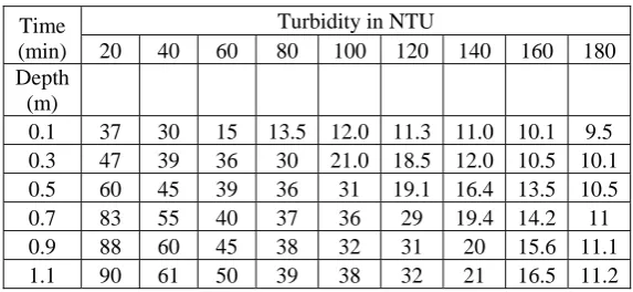
Graph 3 Linear Regression for Graph & Modified Method
Linear Regression through origin for Alum Y = B * X
Parameter Value Error
---B 0.98914 0.00364
---R SD N P
---0.99449 1.26606 18 <0.0001 ---% Rem ov al Ef fi ciency by M o dif ied M et h od
% Removal Efficiency by Graph Method
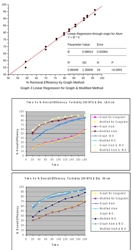
T i m e V s % O v e r a l l E f f i c i e n c y T u r b i d i t y 1 5 0 N T U & D i a . 1 8 . 5 c m
0 1 0 2 0 3 0 4 0 5 0 6 0 7 0 8 0 9 0 1 0 0
0 2 0 4 0 6 0 8 0 1 0 0 1 2 0 1 4 0 1 6 0 1 8 0
T i m e
% O ver al l E ff ici en cy
G r a p h N o C o a g u la n t M o d if ie d N o C o a g u la n t G r a p h A lu m M o d if ie d A lu m G r a p h M . O M o d if ie d M . O G r a p h A lu m & M . O M o d if ie d A lu m & M . O
T im e V s % O v e r a l l E f f i c i e n c y T u r b i d i t y 1 5 0 N T U & D i a . 3 0 c m
0 1 0 2 0 3 0 4 0 5 0 6 0 7 0 8 0 9 0 1 0 0
0 2 0 4 0 6 0 8 0 1 0 0 1 2 0 1 4 0 1 6 0 1 8 0
T i m e
% O v er a ll E ff ici en c y
T i m e V s % O v e r a ll E f f i c ie n c y T u r b i d it y 4 5 0 N T U & D i a . 1 8 . 5 c m 0 1 0 2 0 3 0 4 0 5 0 6 0 7 0 8 0 9 0 1 0 0
0 2 0 4 0 6 0 8 0 1 0 0 1 2 0 1 4 0 1 6 0 1 8 0
T i m e
% O v er a ll Ef fi ci e n c y
G r a p h N o C o a g u la n t M o d if ie d N o C o a g u la n t G r a p h A lu m M o d if ie d A lu m G r a p h M .O . M o d if ie d M . O . G r a p h A lu m & M .O . M o d if ie d A lu m & M . O .
T im e V s % O v e r a l l E f f ic i e n c y T u r b i d i t y 4 5 0 N T U & D i a . 3 0 c m
0 1 0 2 0 3 0 4 0 5 0 6 0 7 0 8 0 9 0 1 0 0
0 2 0 4 0 6 0 8 0 1 0 0 1 2 0 1 4 0 1 6 0 1 8 0
T im e
% O ver a ll E ff ici e n c y
G r a p h N o C a g u la n t M o d if ie d N o C a g u la n t G r a p h A lu m M o d if ie d A lu m G r a p h M .O . M o d if ie d M . O . G r a p h A lu m & M . O . M o d if ie d A lu m & M . O
T i m e V s % O v e r a l l E f f i c i e n c y T u r b i d i t y 1 0 0 0 N T U & D i a . 1 8 . 5 c m
0 1 0 2 0 3 0 4 0 5 0 6 0 7 0 8 0 9 0 1 0 0
0 2 0 4 0 6 0 8 0 1 0 0 1 2 0 1 4 0 1 6 0 1 8 0
T i m e
% O v er al l E ff ici e n c y
G r a p h N o C o a g u la n t M o d if ie d N o C o a g u la n t G r a p h A lu m M o d if ie d A lu m G r a p h M . O M o d if ie d M . O . G r a p h A lu m & M . O . M o d if ie d A lu m & M . O .
T im e V s % O v e r a ll E f f ic i e n c y T u r b id i t y 1 0 0 0 N T U & D ia . 3 0 c m
0 1 0 2 0 3 0 4 0 5 0 6 0 7 0 8 0 9 0 1 0 0
0 2 0 4 0 6 0 8 0 1 0 0 1 2 0 1 4 0 1 6 0 1 8 0
T i m e
% O ve ral l E ff ici en c y
S e r ie s 1 0 G r a p h N o C o a g u la n t M o d if ie d N o C o a g u la n t G r a p h A lu m M o d if ie d A lu m G r a p h M .O . M o d if ie d M . O . G r a p h A lu m & M . O . M o d if ie d A lu m & M . O .
The graphs percent removal vs. detention time is constructed as shown in graph 7 and from these graphs overall removal efficiency is calculated at constant time interval by graphical Method. The overall removal efficiency at constant time interval is calculated by using the formula as follows
R = r0 + (1/H)*{h1*(R6-R5) +h2*(R5-R4) +h3*(R4-R3)} = 75 + (1/1.1)*{0.09(100-90) + 0.34*(90-80) + 0.77*(80-75)} = 82.45 %
Also the Overall Removal Efficiency is calculated by Modified Average Method as follows Removal Efficiency R at time 100 min.
R = Average of percentage removal Turbidity at time t. R = ( 92 + 86 +79.5 +75.7+ 78.7+75) / 6
= 81.1 %
4. Discussion
In this Study the overall removal efficiency is calculated using the Modified average Method and this Modified Method is Verified by comparing the values of overall removal efficiency calculated from Modified average Method and by Graphical Method. From the graph 2 it is observed that the results obtained using this method was similar or very closer to the graphical traditional method. Only 1 % or 2 % of variation occurred some times.
P. Krishnan was Developed this Average Method first time , But he was applied this Method on suspended solid concentration readings measured from the sampling depth of column as we know finding the suspended solid concentration is very lengthy and complicated method and consumes lot of time and will not get the accurate results. Also this method was applied to other available data of various researcher, it gives variation in the Results of overall removal efficiency. Due to these Disadvantages of this Method, some modification is made in the methodology. And the New Modified average Method is Developed. Only the Methodology is changed this Method is applied to the measured turbidity readings obtained from the sampling depth the of settling column. This Modified average Method gives very quick and much accurate results of overall removal as compared to Krishnan Method.
Also Linear Regression analysis was carried out for verification of this modified Method. All the values of overall removal efficiency obtained from both the methods are used for Linear Regression analysis. The Linear Regression graphs for Alum coagulant was shown in the graph 3. The Correlation Coefficient Rc is found out for Alum coagulant it is coming 0 .99, means all values of overall removal efficiency obtained from the modified method are very close to values of overall removal efficiency obtained from the Graph Method.
5. Summary and Conclusion
The Modified average method is developed for overall removal efficiency. This is new methodology for analysis of column settling data. Necessity to develop this new method because of some draw backs of old graphical Method such as the accuracy of the result developed in the old traditional graphical method depends to the great extent on the development of isopercentage lines it is time consuming & tedious. The actual data obtained during experiment is loosed while developing the of isopercentage lines. The isopercentage lines are often drawn as a Line which is best fit, because of the scatter of the data from the column settling which results in the variation in overflow rates, settling velocity, detention time and suspended solids removal.
To eliminate the subjective nature of the development of isopercentage lines. This new Modified Average Method is suggested as simplified method where there is no need for the development of isopercentage lines. Percentage turbidity removal data collected at various column depths for each sampling period can be directly used to obtain the average turbidity removal in the column. The results obtained using this method was similar or very closer to the graphical traditional method. The Verification of this Method is carried out using the Linear Regression analysis.
Acknowledgments
The authors acknowledge the financial help provided by Pune University under BCUD Research scheme 2009-10.
References
[1] Alphonse E. Zanoni and Marshal W. Blomquist (June 1975), “Column settling test for flocculant suspension”.Journal of
Environmental Engg., ASCE, Vol. 101(3), 309 318.
[2] Krishnan (Feb 1976), “Column Settling test for locculant suspension”. Journal of Engg. Div., EE1, 227-229.
[3] Paul M. Berthouex, and David K. Stevens, (Oct 1982), “Computer analysis of settling data”. Journal of Environmental Engg.,
Div.ASCE, Vol. 108(5), 1065-1069.
[4] Peavey S. H., Donald R. Rowe and George Tchobanoglous (1985), Environmental engineering, McGraw–Hill, New York, 121–123
[6] G. K. Agarwal and Desh Deepak (1986), “High rate settling of flocculant slurrys”. Indian Journal of Environmental Health. Vol. 28, Issue No. 4, 314-323.
[7] P. Nema, N. C. Kankal, B. H. Gokhe, C. G. Mehta, (1987), “Evaluation of settling analysis method”. Indian Journal ofEnvironmental
Health. Vol. 33, Issue No. 1, 51-58.
[8] Hasan Ali San (1989), “Analytical approach for evaluation of settling data”. Journal of Environmental Engg., Div. ASCE, Vol. 115(2),
455-461.
[9] D. S. Bhargava & K. Rajagopal (1990), “Modelling in Zone setlling For different ypes of suspended Materials” University of Roorkee.
India.
[10] D.S.Bhargava & K. Rajagopal, (1991), “Settlable studies on sugar mill waste”. Indian Journal of Environmental Health. Vol. 33,Issue
No.1, 51-58.
[11] P. Udaya Bhaskar, Sanjeev Chaudhari and Mohammad Jawed (1992), “Type-II Sedimentation : Removal Efficiency from
column-Settling Test”. Journal of Environmental Engg. ASCE Vol.. 118(3), 757-760.
[12] Viessman W. Jr. and Hammer. M. J. (1998), Water supply and pollution control, Addison-Wesley, Menlo Park, Calif., 370–371.
[13] Waseem Akhtar, Muhammad Rauf, Iqbal Ali and Nayeemuddin (Nov.2004), “Optimum design of sedimentation tanks based on
settling characteristics of karachi tannery wastes”. Journal of water air and soil pollution, vol. 98, 199-211.
[14] Thomous J. Overcamp (Jan 2006), “Type II settling data analysis”, Journal of Environmental Engg., ASCE, Vol. 132, 137-139.
[15] G. R. Bidhendi, A. Torabian, H. Ehsani, N. Razmkhah, (Jan 2006),”Evaluation of industrial dying wastewater treatment with coagulant
and polyelectrolyte as a coagulant aid”. Iran Journal of environmental health science Engg., Vol. 4, No. 1, 29-36.
[16] S.C Ng, S. Katayon, M.J Megat Mohd. Noor and A.G.L. Abdullah, (2006), “The Effectiveness Of Moringa Oleifera As Primary
Coagulant In High-Rate Settling Pilot Scale Water Treatment Plant”. International Journal of Engineering and Technology, Vol.3, No. 2, 2006, pp. 191-200.
[17] O.S. Amudaa, A. Alade, (2006), “Coagulation/flocculation process in the treatment of abattoir wastewater”. Desalination 196, 22–31
Muhammad Saleem, (Apr 2007), “Pharmaceutical Wastewater Treatment: A Physicochemical Study” Journal of Research
[18] (Science), Bahauddin Zakariya University, Multan, Pakistan. Vol. 18, No. 2, April 2007, pp. 125-134
[19] Avid Banihashemi, Mohammad Reza Alavi Moghadam, Reza Maknoon and Manouchehr Nikazar, (Feb 2008), “Development Of A