http://www.sciencepublishinggroup.com/j/ijsda doi: 10.11648/j.ijsd.20170304.13
ISSN: 2472-3487 (Print); ISSN: 2472-3509 (Online)
Imputation Methods for Longitudinal Data: A Comparative
Study
Ahmed Mahmoud Gad
1, Rania Hassan Mohamed Abdelkhalek
21
Statistics Department, Faculty of Economics and Political Science, Cairo University, Cairo, Egypt 2
Department Statistics, Mathematics and Insurance, Faculty of Commerce, Benha University, Benha, Egypt
Email address:
[email protected] (A. M. Gad), [email protected] (R. H. M. Abdelkhalek)
To cite this article:
Ahmed Mahmoud Gad, Rania Hassan Mohamed Abdelkhalek. Imputation Methods for Longitudinal Data: A Comparative Study.
International Journal of Statistical Distributions and Applications. Vol. 3, No. 4, 2017, pp. 72-80. doi: 10.11648/j.ijsd.20170304.13
Received: March 5, 2017; Accepted: March 28, 2017; Published: November 10, 2017
Abstract:
Longitudinal studies play an important role in scientific researches. The defining characteristic of the longitudinal studies is that observations are collected from each subject repeatedly over time, or under different conditions. Missing values are common in longitudinal studies. The presence of missing values is always a fundamental challenge since it produces potential bias, even in well controlled conditions. Three different missing data mechanisms are defined; missing completely at random (MCAR), missing at random (MAR) and missing not at random (MNAR). Several imputation methods have been developed in literature to handle missing values in longitudinal data. The most commonly used imputation methods include complete case analysis (CCA), mean imputation (Mean), last observation carried forward (LOCF), hot deck (HOT), regression imputation (Regress), K-nearest neighbor (KNN), The expectation maximization (EM) algorithm, and multiple imputation (MI). In this article, a comparative study is conducted to investigate the efficiency of these eight imputation methods under different missing data mechanisms. The comparison is conducted through simulation study. It is concluded that the MI method is the most effective method as it has the least standard errors. The EM algorithm has the largest relative bias. The different methods are also compared via real data application.Keywords: Dropout Missing, Longitudinal Data, Missing Data, Multiple Imputations, Single Imputation
1. Introduction
Longitudinal studies become an increasingly common research area especially in the field of public health and medical sciences. Such studies are designed to investigate changes in a specific variable, which is measured repeatedly either at different times or under different conditions. Missing values are common in longitudinal studies because some individuals may miss a planned visit. There are many possible causes leading to missing values including failure of measurement, accidents, errors resulted from collecting or entering data, refusal to continue, or other administrative reasons. Whenever there are missing values, there is loss of information, which causes reduction in efficiency. Also, under certain circumstances, missing data can introduce bias and thereby lead to misleading inferences about the parameters.
Missing data can be classified, based on the occurrence in time, into two patterns: intermittent pattern and dropout
pattern. The intermittent missingness, also termed as non-monotone, means missing values due to occasionally omission, with observed values afterwards. The dropout pattern, also termed monotone, where missing values due to premature withdrawal, with no observed values afterwards (Gad and Ahmed [8]).
Several statistical approaches have been applied to the analysis of longitudinal data with missing values. These approaches should be selected based on the amount of missingness and the missingness mechanism. Some statistical methods are valid only under certain situations with specified missing rates. In other words, there is no unique best method available for all situations. Little and Rubin [12] reviewed many traditional approaches for dealing with missing data and concluded that these methods are only appropriate under the strong assumption of MCAR mechanism. However, in practice the MAR mechanism is much more common than the MCAR mechanism. When the size of the dataset is large enough, analysis can be conducted using deletion methods such as the complete case analysis (CCA) method. The CCA can be used for any statistical analysis and does not need special computations since it is a default method in most statistical computer packages. However, ignoring missing values even in this situation leads to loss of information and reduction of statistical power, which may result in incorrect statistical inference.
Imputation methods are considered as alternatives to the deletion methods. The term imputation means replacing missing values by other observed values or estimated values (Rubin [21]). However, even when an imputed value is closer to an ideal predicted observation; it is still considered as imputed data, not real data. The rule of thumb suggests that 20% or less of missing data is acceptable rate to use imputation methods (Little and Rubin [12]). The imputation techniques can be classified according to the number of imputed values as single imputation (SI) and multiple imputations (MI) methods. In SI techniques each missing observation is replaced by a single value. In MI techniques each missing value is substituted by two or more acceptable values to account for the uncertainty inherent in the imputation process (Rubin [21]).
Many simulation studies have been conducted in literature to evaluate the efficiency of different imputation methods, see for example Engels and Diehr [6], Mishra and Khare [14], Nakai [16], Nakia and Ke [18], Nakai et al. [17] and Zhu [28].
The main purpose of this article is to compare the performance of eight imputation methods. This is accomplished by a simulation study using different missingness mechanisms (MCAR, MAR, and MNAR) with various missingness rates. For simplicity, and without loss of generality, a monotone pattern of missing data is assumed. The performance of imputation methods is evaluated using two criteria; the relative bias (RB) and the mean squared error (MSE). The rest of the article is organized as follows. In Section 2, the basic notations are described. In Section 3, different imputation approaches of handling missing data are reviewed. In Section 4, a simulation study is presented to compare the eight imputation methods. In Section 5, the selected imputation methods are applied to a data set concerning quality of life among breast cancer patients in a clinical trial controlled by the International Breast Cancer Study Group. Finally, Section 6 is devoted to conclusions and
discussions.
2. Notation
For a longitudinal dataset with balanced design all subjects have complete measurements and are measured on the same time points. The main interest is on the relationship between the response variable and some covariates. Unbalanced longitudinal data are possible when some values are intermittently missing or drop out from the data. The repeated measures are potentially observed on the
i
th subject at jth time points tij(
i=1,…, ;m j=1,…,ni)
and the totalnumber of observations is N= . m
i i
n
∑
Yij represent therepeated response variables of subject i, and
(
1, ,)
ij ij ijp
X = X … X are covariates or explanatory variables.
The yij denotes the value of the variable Yij and xijk denotes
the value of Xijk recorded at time
(
1, ; 1, , ; 1, ,)
.ij i
t i= …m j= … n k= … p The
(
)
1, i T
i i in
Y = y …y
is a vector of values for the repeated measures and
i i ijk n p
X x
×
= is a matrix of values of varying or
time-independent covariates on the
i
th subject.3. Imputation Methods
Imputation methods are used to compensate for the unit with missing values. Imputation methods become important in statistical analysis of incomplete data. Some methods use only information that belongs to the subject whose data were missing, while some used the values of other subjects. Imputation methods are classified based on the number of imputed values in place of missing values into single or multiple imputations. In single imputation, each missing value is imputed with a single value while in multiple each missing value is substituted with multiple values producing several different complete datasets. The eight imputation methods are reviewed in this section.
3.1. The Complete Case Analysis Method (CCA)
The CCA is easy and straightforward technique to handle missing data. This method excludes all subjects, in the dataset, with one or more missing values at any measurement occasion. Only cases having complete observations are considered. The CCA method can be used for any type of statistical analysis and does not need special computations since it is the default method in most statistical computer packages.
the complete case dataset (Nakai [15]). When the missing data mechanism is not MCAR, the results from the CCA method may be biased because the complete cases become unrepresentative to the full population (Nakai et al. [17]). Therefore, when the data is MCAR and only a small proportion of units are excluded, this method can be a sensible choice.
3.2. The Mean Substitution Method (MS)
Based on mean imputation method, the mean of the variable is considered the best estimate of any subject who has missing value for that variable. The mean value of non-missing observations is used to fill in missing values for all observations. Although mean substitution maintains the same sample size from reduction, it has some challenges. When data contains fairly large missingness rate, the mean imputation method can distort the distribution of the variable because the possible extreme values are shifted to the middle of the distribution which may complicate the analysis and results in underestimation of the variance which may cause large kurtosis (Little and Rubin [12]). The covariance also is underestimated because the mean imputation for the missing subjects has zero variance. In addition, this imputation method similar to the CCA; it requires MCAR assumption to obtain unbiased and efficient estimates but this assumption is very restrictive.
3.3. The Last Observation Carried Forward Method (LOCF)
The LOCF method is a very common approach for handling missing data especially in dropout missingness (Saha and Jones [22]). This method imputes the unobserved value by the last observed value for the same subject. For dropout missingness, it is assumed that the last observed value is carried forward to the end of the study. This implies that the last observation remains the same after dropout. The LOCF can also be applied to longitudinal data where the subjects are observed at several occasions, and some subjects are lost-to-follow up or have intermittent missing values. This situation could be considered as unrealistic in many settings. The LOCF method tends to underestimate the true variability of the data.
It is shown that LOCF method does not give valid analyses if the missingness mechanism is not MCAR (Lane [11]). However, it creates bias even if the strong MCAR assumption is satisfied. The LOCF can give satisfactory results, if the observations in the dataset are approximately close to each other. When the measurements occasions are short to some extent, this ensures the effectiveness of the LOCF method.
3.4. The Hot Deck (HOT) Method
This method proposed by Madow et al. [13] in which any missing value of unit is replaced by a similar responding unit in the same sample. The responding unit is chosen randomly or selected on the basis of similarity criteria. In the case of more than one similar subject to the subject which contain
the missing values in the sample, the most similar subject is selected and replace the missing values from his or her measurements. Also, in this method the missing value may be filled based on the correlation among the variable containing missing data and the other variables which has no missing.
This method performs well when the variable used to sort the data is highly predictive of the variable with the missing values and when there is a large sample to ensure easily identifying a similar case (Streiner [25]). The hot deck method does not distort the distribution of the sampled values besides the conceptual simplicity of applying it. In addition, using a similarity criterion is a realistic matter and preserves some of the measurement error that would likely be found if the value had been completed by the respondent. Based on the hot deck method, the standard deviation of the variable with the inserted values is a better approximate to the standard deviation value for the variable without the substituted values. However, standard deviations are still likely to be lower (Streiner [25]). It has some cautions like distorting of both correlations and covariance because the missing values are replaced with values that already exist in the distribution of scores. The smaller standard errors lead to greater likelihood of a Type I error (Nakai and Ke [18]).
3.5. The K-Nearest Neighbors (KNN) Method
According to the KNN method, each imputed value is selected from the respondent who is the nearest to the subject with missing value based on the distance between them. The distance is computed using the information from the observed data. The KNN imputation method is appropriate only when the missingness mechanism is MCAR. If MCAR assumption is violated, this leads to biased results. Also, Rancourt et al. [20] stated that the mean estimates are unbiased using the KNN assuming the ignorable missingness mechanism. This method has some nice features (Chen and Shao [3]). First, it is a hot deck method in the sense that donors are substituted by a value from the same variable for a respondent of the same sample. The imputed values are actually occurring values, and they may not be perfect substitutes, but are unlikely to be nonsensical values. Second, the KNN method may be more efficient than the mean imputation method, since it makes use of auxiliary information provided by the x−values and it is a nonrandom imputation method. However, it does not use an explicit model relating y
and x, hence, it is expected to be more robust against model violations than other methods which are based on explicit models. Finally, the KNN method provides asymptotically valid distribution. Rancourt et al [20] stated that the KNN imputation yields normally point estimates with small or negligible bias, assuming that a linear relationship exists between the variable of interest y and the concomitant variable x used for nearest neighbor identified. But this claim was not supported by any theoretical result in general.
3.6. The Regression Imputation (Regress) Method
conditional mean imputation. The basic idea behind regression method is identifying several predictors for the variable with missing values using a correlation matrix. The best predictors (the highest correlations) are selected and used as independent variables in a regression equation. The variable with missing data is used as a dependent variable. This variable is regressed on all other variables to produce a regression equation on the basis of the subjects with complete data for the predictor variables. The regression equation is then used to replace missing values for incomplete subjects with the predicted values. In an iterative process, the values for the missing variable are inserted and then all subjects are used to predict the dependent variable. These steps are repeated until there is little difference between the predicted values from one step to the next, that is, they converge. The predictors from the last round are the ones which are used to replace the missing values (Saunders et al.
[23]). Regression assigns the subject’s predicted value to the missing value but subjects with the same covariates will exactly have the same imputed value (Engel and Diehr [6]).
This method can yield consistent estimates for the mean under normality and MCAR assumption for the missing mechanism but, the sample covariance is underestimated (Little and Rubin [12]). Also, Allison [1] pointed out that regression parameter estimates based on regression imputation under MCAR are relatively unbiased in large samples. However, it has two problems stemming from the fact that the imputed values were perfectly predicted from other variables, they tend to fit a regression line together too well. First, they do not reflect the random error or variance so, the variance of the imputed value of the data set is underestimated which lead to small standard errors and p-values at the time of analysis. Second, the correlations with the imputed variables are overestimated because the underestimated variance of the imputed variable is in the denominator of the correlation formula (Allison [1]).
3.7. The Expectation Maximization (EM) Algorithm
The EM algorithm is introduced by Dempster et al. [4] and implemented for many missing data problems. It is an iterative algorithm that finds the parameters which maximize the log-likelihood function when there are missing values in the dataset. The EM algorithm is carried out through two steps: the expectation step (E-step) and the maximization step (M-step). Given the current parameter estimates, the E-step calculates the conditional expectation of the complete data log-likelihood given the observed data and the current set of parameter estimates. The E-Step can be expressed symbolically (Nakai [15]) as follows:
( )
| ˆ(
|)
| , ˆobs Q θ θ =E g θ Y Y θ θ=
(
|)
(
| , ˆ)
mis obs mis g θ Y f Y Y θ θ dY
=
∫
=where is an estimate for
θ
andg(
θ
|Y)
is the complete data log-likelihood.Given the complete data log-likelihood, the M-step finds
the parameter estimates that maximize the complete data log-likelihood produced from the E-step to obtain updated parameter estimates. The M- step can be expressed (Nakai [15]) as follows:
(
t 1| ˆ) ( )
| ˆQ θ+ θ ≥Q θ θ for all
θ
The iteration between M-steps and E-steps are continued until some convergence is met, that is until values that are re-estimated by the second step approximate the previous estimated values. Many advantages have been reported to the EM algorithm. First, the observed data likelihood increases at every step. Second, the EM algorithm is preferred to regression imputation because the estimated parameter values that maximize the observed data log-likelihood function are consistent, efficient under MAR condition and tend to be approximately unbiased in large samples and normally distributed (Fichman and Cummings [7]). Third, the obtained variances are close to what is theoretically desirable (Dragset [5]). However, the convergence of the iterations can be very slow in case of large fractions of missing data (Nakai and Ke [18]).
3.8. The Multiple Imputation (MI) Method
Multiple imputations method is considered as a continuation to single imputation method from the conditional distribution. The MI approach involves imputing each missing value by two or more acceptable values to produce several different complete datasets. Then each dataset is analyzed to produce different parameter estimates. The sets of parameter estimates from each imputation are then combined using a special rule (maybe by taking the average) to give an overall (single) estimate of the complete data parameters as well as reasonable estimates of standard errors that incorporate the variability in results between the imputed datasets.
example, imputing 5 to 10 datasets cost time, cause computational difficulty, and need testing models for each data set separately (Shieh [24]) Fourth, the MI does not satisfy normality test in most situations (Nakai [16]). Finally, although each of the imputations used in the MI procedure based on regression parameters from the observed data and it is assumed that these regression imputation parameters are the true population parameters, but in fact they are only sample estimates from a sample distribution. Therefore, when multiple imputation methods are implemented, it is preferable to use new parameters drawn randomly for each imputation from a Bayesian posterior distribution of regression imputation parameters rather than using the sample regression parameters for each imputation (Newman [10]).
4. Simulation Study
4.1. Simulation Setting
The aim of this simulation is to evaluate the behavior of eight imputation methods under the three missing data mechanisms. It is based on a dataset for subjects with five measurement times. The sample size n,is chosen to range from small to large. We consider the sample sizes
10, 50,
n= n= and = 100 to represent small, moderate and, large sample sizes respectively. It is assumed that there are two covariates; the time “TIME” and the treatment group “Grp”. Hence the data are simulated according to the following model
0 1 2
ij j i ij
y =
β β
+ Time +β
Grp +ε
where Timej was coded 0, 1, 2, 3, 4 for the five time points,
and Grpiis a dummy variable takes the value 0 for placebo
group and value 1 for treatment group. The simple linear regression model for the mean profiles of the repeated measurements Ε
( )
yij =µj,j=0,1, 2, 3, 4 is used. Thevariance-covariance structure is assumed as first-order autoregressive AR (1). The parameters are fixed at
0 1, 1 0.25,and 2 1
β = β = β = − . The εi's were generated
from a multivariate normal with zero mean and 2
( ij) 1.
V
ε
=σ
= The mean response is( )
yij β0 β1Timej β2GrpiΕ = + + and the (co) variance for
time points
j
and j′equalsσ ρ
2 j−j′, forρ ≥
0
andσ
2is the error variance. The data are simulated to satisfy themultivariate normal distribution and the correlations between two variables Yij and Yij′ . The correlation coefficient is
assumed as = 0.5. The AR (1) structure is
2 3 4
2 3
2 2 2
3 2
4 3 2
1 1
1 1
1
ρ ρ ρ ρ
ρ ρ ρ ρ
σ ρ ρ ρ ρ
ρ ρ ρ ρ
ρ ρ ρ ρ
In general, generating each dataset is based on the following assumption:
1.The measurement at the first time point
( )
t=1 is fully observed,2.The missingness data mechanism are MCAR, MAR and MNAR,
3.The missingness pattern is monotone, and 4.The number of replications is fixed at 5000.
The comparison between methods depends on two measures; the Relative Bias (RB) and Mean Square Error (MSE).
The GLS method is used for estimating the unknown parameters in the linear regression model. The parameter estimates have been obtained for the selected imputation methods: the CCA, the Mean, the LOCF, the HOT, the RM, the KNN, the EM, and MI methods.
For the MCAR situation, the data are simulated with dropout rates of 0%, 25%, 50%, 75%, and 87.5% at time points 0, 1, 2, 3, 4 respectively. If subject is missing at a given time point, then it is considered missing at all latter time points. These rates indicate the percentages of the original sample that are missing at each time point. For the MAR setting, if the value of the dependent variable is greater than the third quartile of the observations, then the subject is dropped out at the next time point. For MNAR setting, after the first time point, if the value of the dependent variable is greater than the third quartile of the observations, then the subject is dropout at that time point and all subsequent time points.
4.2. Simulation Results
The simulation results are presented in Table 1 to Table 9. The MSE results are not presented for the sake of parsimony, but their qualitative conclusions are discussed. It is noted, for all methods, that the relative bias has a negative relation with the sample size. The behavior of the different methods is discussed below.
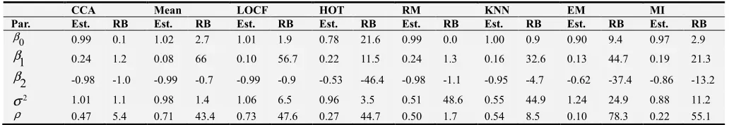
Table 1. The RB% and the MSE of the estimates under MCAR missingness at 0%, 25%, 50%, 75%, and 87.5% missingness rates with n=10.
CCA Mean LOCF HOT RM KNN EM MI
Par. Est. RB Est. RB Est. RB Est. RB Est. RB Est. RB Est. RB Est. RB
0
β 0.99 0.1 1.02 2.7 1.01 1.9 0.78 21.6 0.99 0.0 1.00 0.9 0.90 9.4 0.97 2.9
1
β 0.24 1.2 0.08 66 0.10 56.7 0.22 11.5 0.24 1.3 0.16 32.6 0.13 44.7 0.19 21.3
2
β -0.98 -1.0 -0.99 -0.7 -0.99 -0.9 -0.53 -46.4 -0.98 -1.1 -0.95 -4.7 -0.62 -37.4 -0.86 -13.2
2
σ 1.01 1.1 0.98 1.4 1.06 6.5 0.96 3.5 0.51 48.6 0.55 44.9 1.24 24.9 0.88 11.2
ρ 0.47 5.4 0.71 43.4 0.73 47.6 0.27 44.7 0.50 1.7 0.54 8.5 0.10 78.3 0.22 55.1
Table 2. The RB% and the MSE of the estimates under MCAR missingness at 0%, 25%, 50%, 75%, and 87.5% missingness rates with n=50.
Method CCA Mean LOCF HOT RM KNN EM MI
Par. Est. RB Est. RB Est. RB Est. RB Est. RB Est. RB Est. RB Est. RB
0
β 1.00 0.3 1.02 2.7 1.02 0.2 0.93 6.3 1.00 0.3 1.01 1.1 0.87 12.9 1.00 0.3
1
β 0.24 0.3 0.08 65.9 0.10 56.2 0.24 2.7 0.24 0.4 0.22 8.6 0.12 50.2 0.24 3.9
2
β -1.00 -0.1 -1.00 0.0 -1.00 0.0 -0.86 -13.4 -1.00 -0.1 -0.99 -0.1 -0.57 -42.6 -0.98 -1.4 2
σ 1.00 0.2 0.98 1.1 1.06 6.2 1.01 1.5 0.55 44.9 0.58 41.3 1.26 26.8 0.96 3.1
ρ 0.49 0.8 0.74 48.3 0.75 0.1 0.35 29.7 0.55 11.9 0.55 10.3 0.15 68.0 0.19 60.4
Table 3. The RB% and the MSE of the estimates under MCAR missingness at 0%, 25%, 50%, 75%, and 87.5% missingness rates with n=100.
Methods CCA Mean LOCF HOT RM KNN EM MI
Par. Est. RB Est. RB Est. RB Est. RB Est. RB Est. RB Est. RB Est. RB
0
β 1.00 0.1 1.02 2.6 1.01 1.9 0.97 2.9 1.00 0.1 1.00 0.6 0.84 15.1 1.00 0.2
1
β 0.24 0.2 0.08 65.9 0.10 56.2 0.24 1.1 0.24 0.2 0.24 3.3 0.13 47.5 0.24 1.7
2
β 0.99 0.1 1.00 0.1 1.00 0.1 0.93 6.3 0.99 0.1 1.00 0.2 0.52 47.2 0.99 0.5
2
σ 0.99 0.1 0.98 1.5 1.05 5.8 1.00 0.6 0.55 44.7 0.58 41.1 1.24 24.8 0.98 1.9
ρ 0.49 0.6 0.74 48.9 0.76 52.1 0.35 28.7 0.56 12.8 0.53 7.1 0.17 65.7 0.19 61.7
The Tables 1-3 show that for all sample sizes both the CCA and the RM methods subdue the other methods in performance for MCAR setting. So, they get the best estimates and the smallest RB and MSE. It is noted that as the sample size increases, the value of both the RB and the MSE decrease for most imputation methods. Both the CCA and the Regress methods predict the missing values very well. They can be used for small samples with small rate of missing values. Moreover they can be applied to large samples with small
percentage of missingness. The MI provides efficient estimates especially for large samples irrespective of underestimating of the variance. The HOT method greatly responds to the increase in the sample size. The Mean, the LOCF, and the KNN methods give reasonable results except in the coefficient of the time covariate ( ). The correlation between each time interval and the adjacent one affects the performance of these methods. Concerning the EM, it is obvious that it could not predict the missing values.
Table 4. The RB% and the MSE of the estimates under MAR missingness at 0%, 25%, 50%, 75%, and 87.5% missingness rates with n=10.
Method CCA Mean LOCF HOT RM KNN EM MI
Par. Est. RB Est. RB Est. RB Est. RB Est. RB Est. RB Est. RB Est. RB
0
β 0.94 5.3 1.04 4.6 0.99 0.8 0.80 19.7 0.93 6.1 0.96 3.2 0.85 14.6 0.91 8.5
1
β 0.47 89.5 0.27 10.6 0.38 54.9 0.37 51.2 0.39 56.2 0.33 32.1 0.28 13.7 0.36 46.9
2
β 1.00 0.0 1.00 0.7 1.00 0.4 0.75 24.8 0.99 0.1 0.99 0.9 0.66 33.5 0.94 5.7
2
σ 1.05 5.6 0.94 5.9 0.91 8.7 1.01 1.4 0.69 30.0 0.72 27.4 1.34 34.8 0.87 12.1
ρ 0.56 12.6 0.54 9.8 0.66 33.4 0.36 26.6 0.51 3.9 0.48 2.5 0.21 56.0 0.30 38.6
Table 5. The RB% and the MSE of the estimates under MAR missingness at 0%, 25%, 50%, 75%, and 87.5% missingness rates with n=50.
Method CCA Mean LOCF HOT RM KNN EM MI
Par. Est. RB Est. RB Est. RB Est. RB Est. RB Est. RB Est. RB Est. RB
0
β 0.94 5.0 1.03 3.2 0.98 1.9 0.87 12.4 0.93 6.8 0.91 8.1 0.88 11.3 0.90 9.4
1
β 0.45 83.8 0.27 10.3 0.38 55.1 0.39 59.3 0.37 51.1 0.38 53.3 0.25 3.2 0.38 53.9
2
β 0.99 0.3 0.99 0.3 0.99 0.4 0.94 5.8 0.99 0.3 0.99 0.2 0.73 26.1 1.00 0.6
2
σ 1.02 2.9 0.94 5.9 0.90 9.0 0.97 2.9 0.72 27.5 0.74 25.4 1.24 24.5 0.95 4.7
ρ 0.58 16.2 0.56 13.4 0.68 36.9 0.41 16.9 0.53 6.4 0.51 2.6 0.24 50.7 0.32 35.8
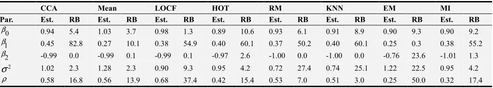
Table 6. The RB% and the MSE of the estimates under MAR missingness at 0%, 25%, 50%, 75%, and 87.5% missingness rates with n=100.
CCA Mean LOCF HOT RM KNN EM MI
Par. Est. RB Est. RB Est. RB Est. RB Est. RB Est. RB Est. RB Est. RB
0
β 0.94 5.4 1.03 3.7 0.98 1.3 0.89 10.6 0.93 6.1 0.91 8.9 0.90 9.3 0.90 9.2
1
β 0.45 82.8 0.27 10.1 0.38 54.9 0.40 60.1 0.37 50.2 0.40 60.1 0.25 0.3 0.38 55.2
2
β -0.99 0.0 -0.99 0.1 -0.99 0.1 -0.97 2.6 -1.00 0.0 -1.00 0.0 -0.76 23.6 -1.01 1.3 2
σ 1.02 2.3 1.28 2.3 0.90 9.3 0.95 4.2 0.72 27.4 0.74 25.1 1.22 22.5 0.95 4.2
According to Tables 4 – 6 the Mean method is superior to other methods for all sample sizes. It is recommended to use the Mean imputation for small sample sizes under the MAR setting. The CCA method indicates also good performance but it does not provide a good estimate forβ1. It is preferable to use the CCA with MCAR setting rather than the MAR
mechanism. All other methods except the Mean and the EM methods sustain from large RB for
β
ˆ .1 The RM, the KNN, and the EM have a bad estimate for the variance. The LOCF, the HOT, the EM, and the MI methods underestimate the value ofρ
. The EM method performs well in the MAR mechanism rather than the MCAR mechanism.Table 7. The RB% and the MSE of the estimates under MNAR missingness at 0%, 25%, 50%, 75%, and 87.5% missingness rates with n=10.
CCA Mean LOCF HOT RM KNN EM MI
Par. Est. RB Est. RB Est. RB Est. RB Est. RB Est. RB Est. RB Est. RB
0
β 0.93 6.6 1.01 1.9 0.97 2.4 0.84 15.5 0.92 7.6 0.95 4.8 0.82 17.3 0.91 8.9
1
β 0.24 1.4 0.06 73.3 0.14 40.1 0.15 37.9 0.22 11.9 0.14 43.4 0.14 43.4 0.19 21.8
2
β -0.83 16.1 -0.82 17.7 -0.83 16.8 -0.48 51.5 -0.80 19.8 -0.75 24.6 -0.50 49.5 -0.74 25.7 2
σ 0.80 19.4 0.68 31.1 0.74 25.2 0.71 28.1 0.48 51.7 0.50 49.3 0.94 5.6 0.68 31.6
ρ 0.50 1.2 0.64 28.6 0.75 50.5 0.29 40.2 0.51 2.7 0.52 5.2 0.22 55.1 0.27 45.1
Table 8. The RB% and the MSE of the estimates under MNAR missingness at 0%, 25%, 50%, 75%, and 87.5% missingness rates with n=50.
CCA Mean LOCF HOT RM KNN EM MI
Par. Est. RB Est. RB Est. RB Est. RB Est. RB Est. RB Est. RB Est. RB
0
β 1.12 12.7 1.14 14.8 1.12 12.7 0.97 2.9 1.13 13.9 1.14 14.2 0.95 4.2 1.06 6.1
1
β 0.09 62.4 0.02 91.7 0.06 72.9 0.03 84.8 0.03 85.1 0.02 90.5 0.06 72.3 0.04 81.2
2
β -0.98 1.7 -0.97 2.5 -0.97 2.9 -0.69 30.8 -0.97 2.4 -0.96 3.4 -0.60 39.2 -0.83 16.5
2
σ 0.96 3.4 0.81 18.8 0.90 9.6 0.78 21.4 0.56 43.9 0.57 42.5 1.12 12.2 0.85 14.5
ρ 0.62 25.2 0.76 53.9 0.80 60.3 0.45 8.4 0.65 30.5 0.68 36.1 0.29 40.3 0.36 26.4
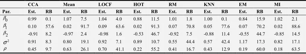
Table 9. The RB% and the MSE of the estimates under MNAR missingness at 0%, 25%, 50%, 75%, and 87.5% missingness rates with n=100.
CCA Mean LOCF HOT RM KNN EM MI
Par. Est. RB Est. RB Est. RB Est. RB Est. RB Est. RB Est. RB Est. RB
0
β 0.99 0.1 1.07 7.5 1.04 4.0 0.88 11.5 1.01 1.8 1.00 0.1 0.84 15.9 1.02 2.1
1
β 0.10 57.6 0.02 91.7 0.09 63.6 0.02 91.3 0.07 70.8 0.05 77.6 0.07 70.2 0.02 88.6 2
β -0.91 8.2 -0.97 2.4 -0.98 1.6 -0.53 46.7 -0.92 7.5 -0.88 11.4 -0.55 44.7 -0.85 14.5
2
σ 0.91 8.3 0.80 19.1 0.92 7.1 0.89 10.7 0.55 44.4 0.57 42.4 1.17 17.3 0.82 17.1
ρ 0.45 9.7 0.63 26.1 0.70 41.1 0.22 55.2 0.41 16.7 0.43 12.9 0.19 60.0 0.18 63.5
Tables 7 - 9 show the results of the MNAR mechanism, in which the estimates are different from the underlying values. It is obvious that the results are impacted by the choice of the missingness mechanism because the methods that performed well in the MCAR and the MAR setting worsen in the MNAR mechanism.
5. Application (Breast Cancer Data)
Breast cancer data concerns with quality of life among breast cancer patients in a clinical trial taken by the International Breast Cancer Study Group (IBCSG). In the IBCSG trial VI (Hurny et al. 1992) premenopausal women with breast cancer are followed for traditional outcomes such as relapse, death and also focused on quality of life. The Patients were chosen at random to represent four groups under four different chemotherapy regimes denoted by A, B, C and D. It is intended to compare the quality of life among the four different treatments.
The patients were asked to complete quality of life questionnaires at baseline (before starting treatment) and at
percentages of patients with 0, 1, 2, 3, 4, 5 missing responses were, respectively, 23%, 18%, 13%, 13%, 14% and 19%. The PACIS measured on a continuous scale from 0 to 100 where, a larger score indicates that greater amount of effort are required for the patient to cope with her illness.
Following Hürny et al. (1992) and Gad and Ahmed (2006) a square-root transformation is used to normalize the data. The averages of the assessments using all available transformed data are 6.1, 5.7, 5.6, 5.1, 4.7, 5.1, respectively, and the standard deviations are 2.50, 2.46, 2.49, 2.51, 2.51, and 2.51. A preliminary version of these data, the responses for the first 9 months of the study, was analyzed by Hürny et al. (1992). Only patients with complete responses are included in the analysis (complete cases analysis). This analysis showed that the treatment differences are not statistically significant. Different versions of these data have been analyzed as Troxel et al. (1998) and Ibrahim et al. (2001)
Gad and Ahmed (2006) adopted the mean model for the responses suggesting the AR (1) covariance structure and the unstructured covariance matrix to analyze this data.
(
)
0 1 1 2logit rij =1 |ψ =ψ ψ+ Yij− +ψ Yij,
for i=1,…382 and
j
=
1,
…
,6.
In this article, we depend on the mean model used in Gad and Ahmed (2006). The response for the first 15 months of the study is determined by PACIS response variable which
are of main interest. The mean model allows each treatment to have its own effect, that is
0 1 1 2 2 3 3, 1, , 6,
j j x x x j
µ
=µ
+α
+α
+α
= …where
µ
0j is a constant shift at each assessment time and(
)
(
)
(
)
(
)
(
)
1 2 3
1, 0, 0 ( )
0,1, 0 ( )
, ,
0, 0,1 ( )
0, 0, 0 ( )
treatment A treatment B x x x
treatment C treatment D
=
The first order autoregressive model is adopted for the covariance structure. In this model the (i, j) th element of the covariance matrix is
σ
ij =2 i j
σ ρ
−for
i j
,
=
1,
…
,6.
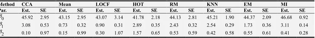
Based on the previous model, a comparison is conducted among different imputation methods to compensate for missing values in the Breast Cancer Data. The standard error is calculated for each imputation method to evaluate the estimator performance.Table 10 displays the estimated parameters using the Generalized Least Square (GLS) method for the eight methods to the Breast Cancer Data. In addition to standard error are calculated to each imputation method for the sake of comparison among them.
Table 10. The parameter estimates of different imputation methods with the values of their standard errors.
Method CCA Mean LOCF HOT RM KNN EM MI
Par. Est. SE Est. SE Est. SE Est. SE Est. SE Est. SE Est. SE Est. SE
0
β 45.92 2.95 43.15 2.95 43.07 3.14 41.78 2.18 44.13 2.81 45.21 1.90 44.37 2.09 46.68 0.92 1
β 3.08 0.53 0.73 0.32 0.90 0.31 2.89 0.35 2.43 0.32 2.54 0.29 1.73 0.36 3.11 0.14
2
β 0.10 0.97 0.15 0.99 0.30 1.07 1.57 0.65 0.53 0.59 0.42 0.58 0.55 0.61 0.41 0.28
The results show that the LOCF method approximately gives the largest standard errors. So, it has the lowest efficiency. In the LOCF method the missing value is replaced with the previous observation. This implies that the imputed value did not predict the missing value well. Unless the values for each time point are close to each other, the LOCF may not be an efficient imputation.
The CCA also shows bad performance. In this method there is much loss of sample size because the subject that has any missing value is removed from the data. Hence, the CCA is recommended for large samples but with small missing values. These data have large number of subjects and high percentage of missing. Moreover, this experiment confirms that the mean imputation is a suitable imputation method when the number of subjects is small and less missing values. The HOT, the Regress, and the EM estimates are approximately close to the mean imputation. They have also large standard errors. It is noted that the KNN method is more efficient than the HOT, the Regress, and the EM methods for this experiment.
The MI method is the most efficient method throughout this experiment. It has the least standard errors value.
6. Conclusion
for the MCAR and the MAR mechanisms. It gets better results as the sample size increase, in other word it should be applied for large sample sizes rather than small sample sizes. The EM algorithm provides a poor prediction to missing values under the three missing data mechanisms especially the MCAR. However, it gives small MSE compared to the other methods. The MI method estimates are relatively biased, but under the MCAR mechanism it has the least bias. The MI method provides small MSE.
Acknowledgements
The authors would like to thank the Editor and anonymous referees for their helpful comments on the manuscript.
References
[1] Allison, P. D. (2002) Missing data, quantitative applications in the social sciences, SAGE University Papers.
[2] Blankers, M., Koeter, M. W. J., and Schippers, G. M. (2010) Missing data approaches in e health research: simulation study and a tutorial for non-mathematically inclined researchers,
Journal of Medical Internet Research, 12, 5: e54.
[3] Chen J, Shao J. (2000) Nearest neighbor imputation for survey data, Journal of Official Statistics, 16, 113–141.
[4] Dempster, A. P., Laird, M. N., and Rubin, D. B. (1977) Maximum likelihood from incomplete data via the EM algorithm, Journal of the Royal Statistical Society, B39, 1-38. [5] Dragset, I. G. (2009) Analysis of longitudinal data with
missing values, MSc. Thesis, Department of Mathematical Sciences, Norwegian University of Science and Technology. [6] Engel, J. M. and Diehr, P. (2003) Imputation of missing
longitudinal data: a comparison of methods, Journal of Clinical Epidemiology, 56, 968-976.
[7] Fichman, M. and Cummings, J. M. (2003) Multiple Imputation for Missing Data: Making the Most of What you Know, Organizational Research Methods, 6, 282-308. [8] Gad, A. M. and Ahmed, A. S. (2006) Analysis of longitudinal
data with intermittent missing values using the stochastic EM algorithm, Computational Statistics & Data Analysis, 50, 2702 – 2714
[9] Hürny, C., Bernhard, J., Gelber, R. D., Coates, A., Gastiglione, M., Isley, M., Dreher, D., peterson, H., Goldhirsch, A. and Senn, H. J. (1992) Quality of life measures for patients receiving adjutant therapy for breast cancer: an international trial, European J. Cancer, 28, 118–124.
[10] Ibrahim, J. G., Chen, M. H. and Lipsitz, S. R. (2001) Missing responses in generalized linear mixed models when the missing data mechanism is nonignorable, Biometrika, 88, 551–564.
[11] Lane, P. (2008) Handling drop-out in longitudinal clinical trial: a comparison of the LOCF and MMRM approaches,
Pharmaceutical Statistics, 7, 93-106.
[12] Little, R. J. A and Rubin, D. B. (2002) Statistical analysis with missing data, 2nd edition, Wiley, US.
[13] Madow W. G., Nisselson, H. and Olkin, I. (1983) Incomplete data in sample surveys, report and case studies, 1, Academic Press, New York.
[14] Mishra, S., and Khare, D. (2014) On comparative performance of multiple imputation methods for moderate to large proportions of missing data in clinical trials: a simulation study,
Journal of Medical Statistics and Informatics, 2, 7662-7669. [15] Nakai, M. (2011) Simulation study: Introduction of imputation
methods for missing data in longitudinal analysis, Applied Mathematical Sciences, 57, 2807-2818.
[16] Nakai, M. (2012) Effectiveness of Imputation Methods for Missing Data in AR (1) Longitudinal Dataset, Int. Journal of Math. Analysis, 6, 1391 – 1394.
[17] Nakai, M., Chen, D. G., Nishimura, K., Miyamoto, Y. (2014) Comparative Study of Four Methods in Missing Value Imputations under Missing Completely at Random Mechanism, Open Journal of Statistics, 4, 27-37.
[18] Nakai, M., and Ke, W. (2011) Review of the Methods for Handling Missing Data in Longitudinal Data Analysis,
International Journal of Mathematical Analysis, 5, 1-13. [19] Newman, D. (2003) Longitudinal modeling with randomly
systematically missing data: A simulation of ad hoc, maximum likelihood, and multiple imputation techniques,
Organizational Research Methods, 6, 328-362.
[20] Rancourt, E., Särndal, C. and Lee, H. (1994) Estimation of the variance in the presence of nearest neighbor imputation,
Survey Research Methods Proceedings, 888-893.
[21] Rubin, D. B. (1987) Multiple Imputation for Nonresponse in Surveys, Wiley, New York.
[22] Saha, C., Jones, M. B. (2009) Bias in the last observation carried forward method under informative dropout, Journal of Statistical Planning and Inference, 139, 246 -255.
[23] Saunders, J. A., Morrow-Howell, N., Spitznagel, E., Dork, P., Proctor, E. K., and Pescarino, R. (2006) Imputing missing data: a comparison of methods for social work researchers,
National Association of Social Workers, 30, 19-31.
[24] Shieh, Y. Y. (2003) Imputation methods on general linear mixed models of longitudinal studies, Committee on Statistical Methodology Conference Papers.
[25] Streiner, D. L. (2002) The case of the missing data: Methods of dealing with dropouts and other research vagaries,
Canadian Journal of Psychiatry, 47, 68-75.
[26] Troxel, A. B., Harrington, D. P., Lipsitz, S. R. (1998) Analysis of longitudinal data with non-ignorable non monotone missing values. Appl. Statist, 47, 425–438.
[27] Van der Heijden, J. M. G., Donders, R. T., Stijnen, T., and Moons, K. G. M. (2006) Imputation of missing values is superior to complete case analysis and the missing-indicator method in multivariable diagnostics research: A clinical example, Journal of Clinical Epidemiology, 59, 1102-1109. [28] Zhu, X. (2015) Comparison of Four Methods for Handing