DOI10.1186/2190-8567-3-11
R E S E A R C H Open Access
A Computational Study of Spike Time Reliability
in Two Types of Threshold Dynamics
Na Yu·Yue-Xian Li·Rachel Kuske
Received: 20 September 2012 / Accepted: 23 April 2013 / Published online: 14 August 2013
© 2013 N. Yu et al.; licensee Springer. This is an Open Access article distributed under the terms of the Creative Commons Attribution License (http://creativecommons.org/licenses/by/2.0), which permits unrestricted use, distribution, and reproduction in any medium, provided the original work is properly cited.
Abstract Spike time reliability (STR) refers to the phenomenon in which repeti-tive applications of a frozen copy of one stochastic signal to a neuron trigger spikes with reliable timing while a constant signal fails to do so. Observed and explored in numerous experimental and theoretical studies, STR is a complex dynamic phe-nomenon depending on the nature of external inputs as well as intrinsic properties of a neuron. The neuron under consideration could be either quiescent or spontaneously spiking in the absence of the external stimulus. Focusing on the situation in which the unstimulated neuron is quiescent but close to a switching point to oscillations, we numerically analyze STR treating each spike occurrence as a time localized event in a model neuron. We study both the averaged properties as well as individual fea-tures of spike-evoking epochs (SEEs). The effects of interactions between spikes is minimized by selecting signals that generate spikes with relatively long interspike intervals (ISIs). Under these conditions, the frequency content of the input signal has little impact on STR. We study two distinct cases, Type I in which thef–I relation (f for frequency,I for applied current) is continuous and Type II where thef–I re-lation exhibits a jump. STR in the two types shows a number of similar features and differ in some others. SEEs that are capable of triggering spikes show great variety in amplitude and time profile. On average, reliable spike timing is associated with an accelerated increase in the “action” of the signal as a threshold for spike generation is approached. Here, “action” is defined as the average amount of current delivered during a fixed time interval. When individual SEEs are studied, however, their time profiles are found important for triggering more precisely timed spikes. The SEEs
N. Yu·Y.-X. Li·R Kuske (
)Department of Mathematics, University of British Columbia, Vancouver, BC, Canada V6T 1Z2 e-mail:[email protected]
Present address:
N. Yu
that have a more favorable time profile are capable of triggering spikes with higher precision even at lower action levels.
Keywords Spike triggered average·Neuronal excitability·Stochastic reliability
1 Introduction
A constant current applied to a neuron at different times usually triggers trains of spikes that do not show reliable timing, due probably to the effects of intrinsic noise and/or differences in the initial state of the neuron when the signal is turned on each time. A stochastically fluctuating signal, however, is capable of generating spikes with remarkably reliable spike timing [1]. This phenomenon has been called spike time reliability (STR) [2], and has been widely observed experimentally in a num-ber of different neurons [1–6] and investigated in several theoretical studies [7–10]. Known as a general property of spiking model neurons [11], STR is closely related to the study of synchronization of uncoupled periodic or chaotic attractors driven by a common noise (see, e.g., [12]).
Given the connection of STR both to the precise mapping of stimuli onto responses and to synchronization, a variety of settings have been explored to better understand the mechanisms and signal features that facilitate STR. For example, gamma range fluctuations have been shown to facilitate the generation of more precisely-timed spikes and induce higher variability in interspike intervals (ISIs) [3]. Effects of the frequency content and the relative amplitude of periodic fluctuations on STR have been investigated in [4,5]. [11] showed that aperiodic inputs, contrary to periodic ones, induced reproducible responses. Reliability in the timing of bursts of action po-tentials can also be achieved through a frozen random input [13]. Galan et al. showed in both experiments and simulations that STR exhibits a local maximum as the cor-relation time of the external input is increased. In an apparently different context of stochastic resonance, a mechanistically related phenomenon was also demonstrated in a summing network of excitable units [14].
oscillations, but these did not consider STR. A computational study using conduc-tance based models compared STR and its precision both in the mean-driven firing range [18], where firing occurs without an external stimulus, and in the fluctuation-driven regime, where firing occurs only with an external stimulus that drives threshold crossing. There the influences of frequency and amplitude of oscillatory stimuli are emphasized, and conditions where impedance profiles may be important were iden-tified. In a recent theoretical study, STR in the case of quiescent neurons is analyzed [19]. There stochastic amplitude and phase equations for two coupled canonical con-ditional oscillators were derived in a subthreshold parameter regime and under the influence of distinct intrinsic noises and a common external stochastic drive. The asymptotic approximations for the probability density of the phase difference re-vealed that, for dominant common extrinsic noise, the phase difference is strongly peaked at zero for comparable intrinsic noise levels or at a nonzero phase difference for different levels of intrinsic noise, indicating synchronized or phase-locked oscil-lations. In addition, the spikes generated by the common external noise could appear irregular and incoherent, yet spike timing is remarkably precise when a frozen copy of the external noisy stimulus is applied, as observed in [1]. In the setting where the neurons are quiescent without an external noisy stimulus, we have not yet seen thorough theoretical or mechanistic explanations for the range of elements that can promote STR. The present study is aimed at revealing some important aspects of such mechanisms using a simple neuronal model.
For a more complete understanding of the STR in a quiescent neuron, in the context of noise-induced irregular and incoherent spiking, it is necessary to deter-mine which features of the input signal are crucial for triggering spikes with precise timing. Spike initiation in a quiescent neuron is often associated with a threshold phenomenon, which happens when a critical transmembrane potential is exceeded. Therefore, spike-triggering can be regarded as a complex “pattern recognition” pro-cess [1], a “feature detection/dimensional reduction” process [20, 21], or even a “time-localized resonance” process, as we view it here and in [22], providing sup-port for this concept in this paper. Mathematical models of neurons are useful tools in exploring these aspects of STR. Unlike real neurons in which the dimensionality and the intrinsic noise are both unknown, the dimension of a model and the intrin-sic noise are well defined in mathematical models. We carry out a computational analysis of the Morris–Lecar model [23], which has only two variables. Both the intrinsic noise and external signals enter through the voltage equation. This model allows an analysis of the threshold of spike-generation in the phase plane in order to investigate previously unexplored aspects of the external stimulus that can sup-port STR. An understanding of both the phase-plane dynamics and bifurcation of the underlying system contributes to the identification of the key elements of the reliable spike-evoking epochs (SEEs) in the signal. The dynamical analysis is particularly im-portant in the context of quiescent neurons, where features like intrinsic frequencies or well-defined regular oscillation are not necessarily contributing factors as they are when the neurons exhibit repetitive firing in the absence of an input signal.
trigger a spike reliably in the presence of different copies of intrinsic noise; and (iii) the potentiation of a time localized temporal epoch in the input that “resonates” with the neuron to trigger a spike reliably at low amplitude. Focusing on these factors allows us to identify the key features of individual spike-evoking epochs (SEEs) that drive reliable spike timing, even though these SEEs show great variety in amplitude and time profile. On average, two specific features are shown to be crucial for reliable spike timing: (1) the accelerated increase in “action” level (defined as the amount of current delivered during a fixed time interval) as the spiking threshold is approached and (2) the time profile of a SEE. The SEEs that have a more favorable time profile trigger more precise spike timing at a reduced level of action. These results are in good agreement with experimental observations [1].
The effects of the three key factors mentioned above are best studied when the effects of other dynamic properties of a neuron are minimized, such as the inter-spike refractory period (IRP) and the intrinsic frequency of an oscillatory neuron. It has been shown that STR is reduced when the frequency of the stimulus-induced re-sponse is high [6], typically due to interference with the IRP or intrinsic frequency. To minimize the influence of IRP and intrinsic frequencies on model neurons that are quiescent in the absence of external inputs, we use specifically generated input signals that only trigger spike trains with relatively long ISIs. An important part of the input signals are spike-triggered averages (STAs), obtained from averaging many time-varying spike-generating stimuli over small time windows preceding the spikes [24]. Using STAs rather than signals with a specific frequency is necessary for our setting, since the dynamics of the quiescent neuron is not associated with a specific intrinsic frequency. In fact, we show that the reliability is insensitive to frequency content of the noisy signal, as long as the ISIs are sufficiently long.
The phase-plane analysis presented here indicates how the combination of action and time profile leads to reliable spike timing in the setting of quiescent neurons. This analysis is complemented by studying both the averages and distributions of properties of the SEEs and the STAs obtained from subsets of the SEEs. Additional important elements are suggested by the characteristics of different subsets of the SEEs that are found to be reliable, such as a time profile that allows the system to “settle” near the steady state while providing sufficient current over a time interval. In combination, these characteristics contribute to the three important factors mentioned above, and increase the precision of the firing over repeated trials.
Furthermore, we see that the underlying bifurcation structure of the neuron, which characterizes its quiescence-to-spiking transition, can also influence the effectiveness of the action-time profile combination. We study two distinct sets of parameter val-ues that give rise to two bifurcation types, and thus two different scenarios of spike transition. Type I is characterized by a gradual increase in the frequency from zero as the bifurcation parameter—here the (base) input current—changes beyond the transi-tion point. Type II is characterized by a jump increase in the oscillatransi-tion frequency as the bifurcation parameter reaches the quiescence-to-spiking transition point (see [25,
contexts, starting with FitzHugh [27], and more recently in the areas of excitability, bursting, and mixed-mode oscillations [28,29]. The relationship of different neuron dynamics to phase plane structures that approximate the firing threshold has been developed as a diagnostic tool to understand variable neuron responses to fluctuating environmental parameters (see, e.g., [30] and references therein). Here, we compare the transitions and the underlying threshold dynamics in the phase plane, to reveal the differences and similarities in the roles that action and time profile play in the two types. For example, in Type I neurons the fluctuations near the slow manifold al-low for reliable spiking transitions over a smaller range of action levels, with greater variation in the precision. Thus, we indicate the role that the bifurcation structure can play in identifying features that support STR.
The remainder of the paper is organized as follows. In the model and methods section, we introduce the Morris–Lecar model that we used in the simulations. We discuss the measure we employed to calculate the reliability of spike timing, as well as the computational methods employed in the simulation and analysis. The main results are presented in the results section that is followed by the discussion section.
2 Model and Methods
2.1 The Model
We use the Morris–Lecar (ML) model [23] in the present study. The noise terms are included additively to the voltage equation.
cdv
dt = −gCam∞(v−vCa)−gKw(v−vK)−gL(v−vL)
+Ibias+δ1η1(t )+Iext, (2.1) dw
dt =λ(v)
w∞(v)−w,
wherev is the membrane voltage potential; w represents the probability of open-ing of K+ channels (0≤w≤1). m∞(v)=0.5(1+tanh((v−v1)/v2)),w∞(v)= 0.5(1+tanh((v−v3)/v4)),λ(v)=φcosh((v−v3)/(2v4)). Here,Ibiasis a base or bias current that is constant in the neuron, typically viewed as the underlying fixed control or bifurcation parameter related to different states in the dynamics. The term δ1η1(t )is the intrinsic noise, whereη1(t )is modeled as a standard Brownian mo-tion, with a distinct realization of the intrinsic noise used on each trial. We refer to the coefficientδ1to indicate the intensity of the intrinsic noise. The termIextis an additional extrinsic current, given byIext=Ic+δ2η2, where the constantIc is just
Table 1 Parameters of Type I and Type II models Shared parameter Different parameters
Values Type I Type II Type I Type II
vK −84 mV gK 8 mS/cm2 5 mS/cm2 Ibias 33 µA/cm2 63 µA/cm2 vL −60 mV gL 2 mS/cm2 3 mS/cm2 ISNIC 37.7 µA/cm2
vCa 120 mV gCa 4.4 mS/cm2 5.6 mS/cm2 ISN 67.31 µA/cm2 c 20 µF/cm2 v3 12 mV −4.5 mV IHB 77.62 µA/cm2 68.05 µA/cm2
v1 −1.2 mV v4 17.4 mV 15 mV τ 7 ms 3 ms
v2 18 mV φ 1/15 ms−1 0.04 ms−1 Ic 4.3 µA/cm2 4.1 µA/cm2
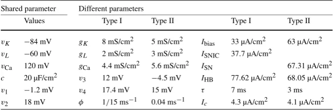
In the absence of noise, the deterministic ML model can be tuned into condi-tions for both a Type I and a Type II neuron. For the Type I parameters listed in Table1, the bifurcation diagram is presented in Fig.1a (top) together with thef– Ibias relationship (bottom). The latter shows a continuous change in the oscillation frequency from zero asIbias increases beyond a SNIC (saddle-node on an invari-ant circle) bifurcation point. The SNIC point is located at ISNIC≈37.7 µA/cm2. For the Type II parameter values, the bifurcation diagram and the f–Ibias rela-tionship are shown in Fig. 1b. A saddle-node (SN) bifurcation on the periodic branch occurs atISN≈67.31 µA/cm2. A subcritical Hopf bifurcation (HB) occurs atIHB=68.05 µA/cm2. The transition from a steady state to an oscillatory state can occur at both the SN and the HB points. The oscillatory solutions that emerge in each case have a finite, nonzero frequency as can be seen in the lower panel of Fig.1b.
The Type I and Type II behaviors with additive noise were studied in [31], where computations of the stationary densities and potential stochastic bifurcations were analyzed. While there are no noise-induced bifurcations in both types, additive noise drives spiking in the excitable regime, where Ibias is below the critical bifurca-tion value and the attracting state is a stable equilibrium. In Type I, the spiking occurs through a coherence-resonance like phenomenon where the excursions fol-low heteroclinic orbits between an equilibrium and a saddle point. The behavior is similar for Type II, but the excursions follow unstable limit cycles. The simula-tions in the present study are carried out under the following condisimula-tions. Near the Type I transition, we picked Ibias =33 µA/cm2 and an external current injection withIc=E[Iext] =4.3 µA/cm2. The total external current,Itot=Ibias+Iext, has
Fig. 1 Bifurcation diagrams and the correspondingf–Ibiasrelationship near a Type I (a) and a Type II (b)
transition in the Morris–Lecar (ML) model.Ibiasis the control parameter. Stable and unstable equilibria
are marked withsolidanddashed lines, respectively. Stable and unstable periodic solutions are marked withfilledandopen circles, respectively. The intrinsic frequency of a steady state is determined by the imaginary part of the eigenvalues of the Jacobian matrix for the corresponding system linearized about the steady state. These diagrams were obtained using the XPPAUT package by Ermentrout [35]
as indicated in the captions of Figs.3,4, and6,7,8. For Fig.5, the signal is composed of SEEs and other epochs that do not trigger a spike, constructed in a way to provide certain spectral properties.
2.2 Computational Methods
2.2.1 A Measure for Spike Time Reliability
In the present study, a correlation based measure [32] is used to determine spike time reliability, which is defined as
R= 2
N (N−1)
N
i=1
N
j=i+1
sisj
| si|| sj|
(2.2)
whereN is the number of trials and si (i=1;. . .;N) are the filtered spike trains,
that is the convolution of the spike train of a trial and a Gaussian filter with a filter width ofσc=20 ms.Rranges from 0 (nonreliability) to 1 (full reliability). This
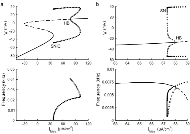
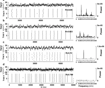
Fig. 2 Raster plots showing spike-time reliability (STR) of the ML model in the Type I conditions (upper panels,a–b) and the Type II conditions (lower panels,c–d). Parameter values used are given in Table1. The coefficientδ1of the intrinsic noise is 5 µA/cm2for (a)–(d), and the coefficientδ2of the external noise
is 0.91 µA/cm2in (b) and (d)
Lyapunov exponent (see, e.g., [9]), used in networks, and the phase measure based on the period of the input [7] used in the self-sustained oscillatory regime, do not suit the context of the fluctuation-driven firing regime studied here.
This reliability measure changes as the numberN changes. However, in simula-tions carried out in this study,R usually settles to a constant level for values ofN larger than 30 (results not shown), with remaining parameters unchanged. Therefore, for eachRvalue, we calculated in the results section, we choseN=45 to ensure that changes inRare not due to changes inN in this range.
2.2.2 Simulation of Stochastic Differential Equations
The stochastic model equations in the present work are numerically solved using MATLAB. To reach a good balance between accuracy and computational efficiency, the fourth-order Runge–Kutta scheme is often used for neuron models. The evolution of the deterministic terms of the equations are calculated using a fourth-order Runge– Kutta scheme with a fixed step of t=1/30 ms, while the influence of the noise terms is renewed at each time step t based on the nature of the noise. Noting that (2.1) has the form
cdv
dt =F (v, w)+Ibias+Ic+δ1η1(t )+δ2η2(t ), dw
dt =G(v, w),
(2.3)
then the increment in theV equation takes the form
Vn+1=Vn+
t
wherekj are the standard contributions from a Runge–Kutta 4 (RK4) [33] method
forV(t )=F (v, w)+Ibias+Ic. The white noise increment η1term is distributed as a Gaussian random variable with mean 0, variance√ t and the increment of the external stochastic signalη2 is the convolution of a white noiseξ and an alpha function,
η2(t )=
∞
0
ξ(t−T )α(T )dT
Then η1is simulated by√ t Z, forZa standard normal random variable and
η2=
∞
0
α(T ) ξ(t−T )dT (2.5)
where ξ is a white noise increment, Gaussian with mean zero, variance t. The increment in thewequation is composed simply of the contributions from the RK4 method, as there are no stochastic contributions there. As noted above,η2is a frozen copy across trials of the stochastic part of the extrinsic input, while the intrinsic noise η1varies from trial to trial.
2.2.3 Computation of Probability Values (p-Values)
p-Values are used to statistically quantify the significant difference of the means of two groups of data in order to determine if the data share the same source [34]. In order to examine characteristics that can be used to differentiate between reliable and unreliable SEEs, we calculate the p-values to measure the average level of differ-ence of “action” levels, as shown in Sect.3.4, using the paired t-test (due to their time-related properties). The p-value measures whether the data from reliable and unreliable SEE is significantly different, with a smallpvalue, normallyp <0.05, in-dicating a small probability that the data from the two classes of SEE’s have the same means. Using the t-test, we also calculated p-values for the values ofwobserved at firing as generated from reliable spikes and unreliable spikes, and the standard devia-tion of the firing times for different subgroups of reliable SEEs, as shown in Sects.3.4
and3.5.
2.2.4 Slow Manifolds and Pseudo-slow Manifolds
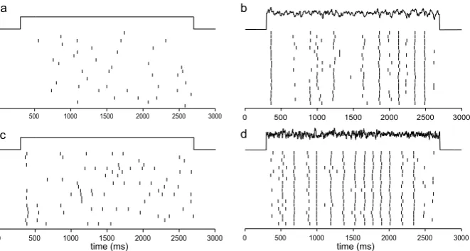
Fig. 3 ReliabilityRof the Type I (a) and Type II (c) ML models is plotted inthe left columnsagainst the SD of the external noise that is either convoluted (solid) or white (dashed).Ris plotted againstτ
for Type I (b) and Type II (d) in
the right columns. Parameter values are given in Table1. The coefficientδ1of the intrinsic
noise is 2 µA/cm2fora–b, and 5 µA/cm2forc–d. The coefficientδ2of the external
noise is 0.91 µA/cm2inband 1.64 µA/cm2ind
into two regions, and the dynamics evolve in opposite directions in the two regions on either side of it. In one region, the trajectories flow to the stable fixed point (i.e., rest potential) quickly without firing; in the other region, the trajectories follow a large excursion (i.e., action potential) before returning back to the stable fixed point. Since XPPAUT plots the trajectories of the Type II model automatically, we chose the trajectory that separates the phase space into two regions as described above as the pseudo-slow manifold. The stochastic stimulus drives the voltage dynamics, so that the voltage nullcline (dV /dt=0) varies with time as does the correspond-ing (pseudo-)slow manifold. Figure6a and c provide snapshots of the (pseudo-)slow manifold when the injected current has different values at different times, as discussed further in Sect.3.4.
3 Results
3.1 Reliability as a Function of Signal Strength and Correlation Time
function ofτ for lower intrinsic frequencies. There is no maximum as a function ofτ for the Type I model, whereRshows a monotonic increase asτ increases (Fig.3b).
When white noise with zero correlation was used instead, good reliability could also be obtained (dashed curves in Figs.3a and c). But a larger SD value is required if one wants to achieve the same level of reliability. This suggests that higher noise intensity helps improve the reliability. However, at identical noise intensity correlated noise leads to higher reliability. An optimal correlation time exists for the Type II model. The mechanism underlying the improved reliability at higher values of the correlation time is not known. However, one potential explanation is provided later in this paper.
3.2 Spike Triggered Averages Are Effective in Triggering Reliable Spikes
The spike triggered averages (STA) are obtained by averaging many time-varying stimuli in a small time window preceding every spiking event [24]. The averaging process over a large population of stochastic stimulation epochs cancels out the tem-porally changing components that a spike does not prefer, leaving the optimal signal for a neuron response. Thus, STAs have been widely used to study the sensory filter properties of neurons in auditory neurons [36,37], electrosensory systems [38,39] and even in visual systems [40,41].
Here, the spike triggered averages (STAs) are calculated for both the Type I and Type II models over a time duration of 100 ms. Specifically,
STA(t )= 1 N
N
i=1
u(t−ti+ STAt )−u(t−ti)
Iext(t ) (3.1)
whereN denotes the number of spikes,ti is the spike time, STAt is the binwidth
of STA, u(t )is the Heaviside unit step function (0 if t <0 and 1 ift ≥0). The STA for each type is calculated using 195 SEEs taken from some test signals. Many copies of the STA for each type are then connected by background fluctuations of different lengths that are not capable of triggering a spike. Figure4shows that the STAs inserted in these background signals are effective in triggering spikes reliably. Special care was taken to guarantee that the average value of these signals is not altered by such connections between pieces of signals.
3.3 The Frequency Content Is not Essential for STR Provided ISIs Are Long
Fig. 4 Spike triggered averages (STAs) for Type I (a) and Type II (c) ML models together with the corresponding response in membrane voltage. Artificial signals are generated (the upper panelinbandd) by connecting many copies of the STA with pieces of background fluctuations of different lengths that are known to be incapable of generating a spike. A typical response of a Type I (b) or a Type II (d) ML model to such a signal is shown in a raster plot. Noise coefficientsδ1andδ2for Type I and Type II are as in
Figs.3b, d. The reliability measureRis calculated and marked in the figure for each type
that the existence of a significant component of the intrinsic frequency in the signal typically enhances the STR through a resonance effect. In the Type I model, no in-trinsic frequency is defined in the vicinity of the SNIC since periodic solutions start with a frequency that is equal to zero. Therefore, we focus on the Type II model. Two intrinsic frequencies can be defined in the vicinity of the Hopf point. The intrinsic frequency of the linearized system forItot=67.1 µA/cm2is 0.00715 kHz. The fre-quency for the stable periodic solution atItot=67.1 µA/cm2is close to 0.00641 kHz. These two frequencies become identical at the HB point in this particular case (see Fig.1b).
Fig. 5 Reliability is insensitive to the frequency content of the noise signal when ISIs are long, shown for Type II. Test noise signals are generated by connecting distinct samples of spike-evoking epochs (SEEs) with intervals of samples that are known to be incapable of generating a spike. The power spectrum for each signal is plotted inthe right panel. From top to bottom, the peak frequency component is located at 0.00641 kHz ina, 0.004 kHz inb, 0.01 kHz inc, and is insignificant ind. The values ofRare calculated with data collected from 100 trials, each containing more than 45 spikes
intrinsic frequency. Reliability remains high in this case although slightly reduced due partly to the shortening of ISIs when the frequency is higher than the intrinsic frequency. In the case shown in Fig.5d, there is no obvious peak in the spectrum when it is plotted using the same vertical scale as in a and b. However, the reliability remains close to 0.8 in this case.
These results suggest that to achieve high reliability in the noise-induced spike train, there is no need for the signal to contain a major fraction of the Fourier compo-nents with frequencies that are near or identical to the intrinsic frequency of either the subthreshold state or the oscillatory state. This result typically applies to the situation when the ISIs in the signal-induced spike trains are relatively long, as in the context of quiescent neurons considered here.
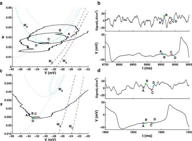
3.4 Reliable SEEs on Average Show Accelerated Increase in Action
Fig. 6 Phase plane trajectories traced out by the responses of the model to two different SEEs (panels
aandc) and the SEEs profiles (top) and the corresponding voltage responses (bottom) (panelsbandd). Four time pointsA,B,C, andDare chosen and the corresponding location of the (pseudo-)slow manifolds (dashed lines)MA,MC, andMDare plotted inaandc.Dotted linesare nullclines whenI=Ibias+Iext.
Note that the location of the pointsA–Dvary around the location of the slow manifold in Type I (top row), while for Type II (bottom row) these values fluctuate less, thus yielding values of the response well below the (pseudo-)slow manifold as the input signal strength increases for Type II. Note in particular that the value ofwfor Type II, pointD, is well below the values on the pseudo-slow manifoldMD. Noise
coefficientsδ1andδ2for Type I and Type II are as in Figs.3b, d
epochs of the signal that trigger a spike with reliable timing from those that cannot? Let us call the SEEs of the signals that reliably drive spiking “reliable SEEs” and those that do not reliably drive spiking the “unreliable SEEs.” We aim to answer the following question. Is there a unique, dominant feature that separates the reliable and unreliable SEEs? The answer to the latter question is probably no, if one examines simply the time series or traces of the two groups SEEs. When a large number of SEEs are examined, they all appear very different from one another, so it is not obvious what features may be appearing more frequently in the reliable SEEs (see for example the two SEEs in Figs.6b, d). However, comparing distributions of key features of the SEEs indicates a direction to partly answer this question.
us to set up a database for both reliable and unreliable SEE pools. A total of 450 reliable SEEs and 600 unreliable ones were collected. This leads us to the study of the following features of each SEE.
We also need to identify a critical threshold for providing a clear identification of the initiation of a spike. For a deterministic Type I neuron, the threshold can be clearly defined in terms of the slow or invariant manifold associated with a saddle point. In contrast, in a Type II neuron this threshold has to be determined by finding a separation of the phase space, dividing those trajectories evolving towards a stable fixed point and those following a larger excursion corresponding to firing. Without sufficient input current, the trajectory can not transition from the quiescent region to the firing region, so the (pseudo-)slow manifold here serves as the firing threshold. Both the slow and pseudo-slow manifolds are found with XPPAUT, as described in Sect.2.2. Since the input current is fluctuating, the (pseudo-)slow manifold is also fluctuating, calculated at a specific time, with the given value of the input at that time. This movement is highlighted in Fig.6where dashed lines indicate the slow (Type I) and pseudo-slow (Type II) manifolds, that shift with fluctuations in the input. It is also useful to identify a working threshold inv only, that can be used to com-pare the behaviors for the two types of neurons. With the presence of noise shifting the (pseudo-)slow manifolds, there is some complication in setting a common value ofvth. For simplicity, we chosevth= −20 mV as this working threshold, where the slope ofv(t )turns significantly positive preceding each spike (see Figs.4a, c), for both Type I and Type II neurons.
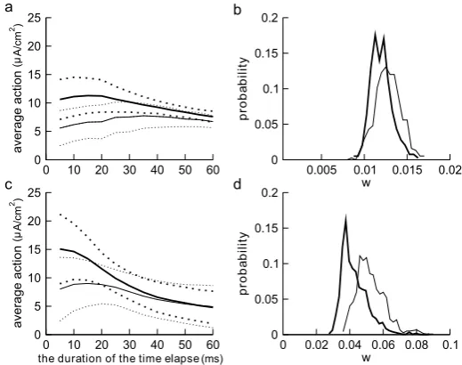
Fig. 7 Average action in progressively shorter time intervals before the spike threshold is reached for both Type I (a) and Type II (c) ML models.The horizontal axisrepresents the duration of time over which action is calculated, starting at the time when spiking threshold is reached. The shorter the time interval, the closer it is to the threshold.The thick solid curverepresents the average action of reliable SEEs and
the thick dotted curvesrepresent the upper and lower limits based on the SD.The thin solid curvedenotes the average action of unreliable SEEs andthe thin dotted curvesmark the upper and lower limits of the SD.The thick solid curvesare averages of 400 reliable SEEs andthe thin solid curvesare averages of 600 unreliable SEEs. The histogram of the values of the gating variablewwhen the reliable (bold line) and unreliable (thin line) spike trajectories pass through the threshold atvth= −20 mV are plotted inb
anddfor Type I and II models, respectively. Noise coefficientsδ1andδ2for Type I and Type II are as in
Figs.3b, d
The increase in action levels of the reliable SEEs (thick curve) continues almost all the way to about 5 ms before reaching the threshold for the Type II model. For this type, the action for the unreliable SEEs (thin curve) also increases as the threshold is approached, reaching a maximum at about 15 ms and starts to decrease for shorter time intervals. For the Type I model, the increase in the thick curve is less steep and reaches a plateau around 15 ms before the spiking threshold. For this type, the thin curve for unreliable SEEs started decreasing at about 35 ms before the spike threshold is reached.
observations [43,44] in which the voltage “threshold” changes with the random gat-ing of the Na+channel. The time series shows the increase invleading to spiking that follows point D, wherewtakes a lower value and the trajectory moves into a range where there is no strong attraction to the fixed point of the underlying deterministic system. The histograms shown in Figs.7b and d suggest that, on average, the value of the gating variablewas the voltage passes through the threshold ofvth= −20 mV is significantly lower for reliable SEEs (thick curve) than that of the unreliable ones (thin curve) for both Type I and II (p <0.01 for both types).
This observation suggests that the unreliable spikes are triggered at larger values ofwon average after spending more time in the close vicinity of the pseudo unstable manifold. Also, there is a larger relative shift between the densities ofwof the reliable and unreliable spikes of Type II, where the difference in means for the two groups is larger than one standard deviation. This result, together with the observations that the response values tend to fluctuate near the slow manifold in Type I and that spiking occurs for slightly lower action values as shown in Fig.7, suggests that the threshold crossing related to firing in the Type I neuron may be more dependent on the signal amplitude. We discuss this further in Sect.3.5, in the context of the standard deviation of firing times.
3.5 The Influence of Time Profiles Revealed by Individual Features of Reliable SEEs
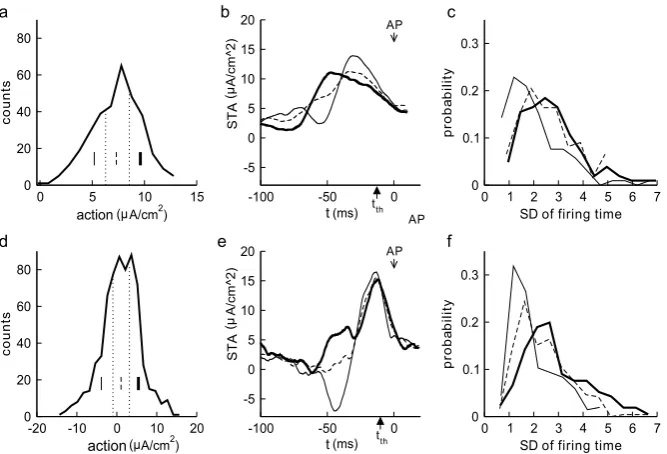
By studying specific examples of reliable SEEs defined above, one realizes immedi-ately that they still appear very different from each other. This motivated us to divide the reliable SEEs further into three subclasses each one third in numbers: the high action, the medium action, and the low action ones (see the histograms Figs.8a, d). The goal is to find out if the time profile of an SEE plays a role in determining the reliability of spike timing and, if the answer is positive, what time profile is more favorable for each type.
Fig. 8 The distributions of action values over a brief time interval of 20 ms for all reliable SEEs. Plotted inaanddare the action distributions for Type I (top row) and Type II (bottom row) models, respectively. The distribution is equally divided into three subclasses. The STA of each subclass is shown inbandewith different line types each marking one subclass as inaandd. The histograms for the standard deviation of the spike times over all 40 trials for each subclass of reliable SEEs, as identified in panelsaandd, are shown incandf. Note that the subclass of reliable SEEs with lower actions typically have smaller standard deviations (SDs) of firing times, thus indicating more closely synchronized spike time reliability. Noise coefficientsδ1andδ2for Type I and Type II are as in Figs.3b, d
Comparison of the precision of the low action SEEs (thin line) and high action SEEs (thick line) show significant differences in the standard deviation of the firing times for both types (p <0.01). Observations about the distribution of the action, time profile, and firing times shown in Fig.8 and time profile in b, e can also be connected with the observations from the phase plane. Time profiles with a downward change can encourage the dynamics to shift toward the steady state, thus settling the response and removing the memory of earlier stimuli. The steep increase of the signal following this downward change then shifts the (pseudo-)slow manifold up, allowing the possibility of a rapid transition to firing. SEEs with high action typically push the response over the firing threshold, but in a way that the dynamics fluctuate around the (pseudo-)slow manifold, resulting in more variation of the location and timing of the transition to firing.
1.5<SD<2 for the subclasses of Type II, as compared with the corresponding Type I subclasses.
The wave form of the thin curves in Figs.8b and e occurs more frequently when an appropriate correlation timeτ is used in the convolution. This brings our discus-sion back to the problem proposed previously. Which features of the SEEs are crucial for STR? The answer is probably a combination of the action level immediately pre-ceding the time when the spiking threshold is reached and a stereotypical wave form of the SEE. We believe the influence of the correlation timeτ is probably indirect, making it more likely for the stereotypical wave form to occur at increasing values ofτ.
4 Discussion
STR is a complex dynamic phenomenon that depends on both the features of the in-put signal and the intrinsic properties of the neuron. In a carefully designed study of spike initiation by a current injection in the form of a Gaussian white noise [1], it was revealed that a wide variety of current wave forms could be effective in triggering a spike reliably. It was therefore concluded that a number of stimulus parameters, in-cluding polarity, amplitude, variability, slope, acceleration, and temporal correlation, are relevant in spike triggering. It was believed that the absence of one feature in one particular spike-evoking epoch (SEE) of an input signal may be compensated for by the presence of another. Temporal profiles of a SEE favorable for precise spike-generation should be related to the dimensionality of the equations required to de-scribe the dynamics of a neuron and the geometric structure of the manifolds in the phase space that define the thresholds beyond which a spike is generated. The na-ture and the magnitude of intrinsic noise also play important roles in the reliability of spike timing. These intrinsic properties of a neuron in an experimental setting are typically unknown. This is where computational models, combined with analysis of dynamical structure and comparison of statistical quantities, are helpful for reveal-ing these properties and potentially the roles of different channels in shapreveal-ing such a favorable profile.
There is a large number of neuronal types where STR has been observed, rang-ing from neocortical neurons [2] to neurons in visual cortex [3], motor neurons [1,
with the goal of revealing some similarities and differences between neurons that dif-fer in threshold dynamics. Although results presented in this work were obtained in a rather simple, two-variable current based model of neurons and with specific additive internal and external noise inputs, the main conclusions are strikingly similar to the experimental data obtained inAplysia californiaabdominal ganglia [1]. The action explanation proposed here is very similar to the experiments in which Gaussian white noise with very different amplitudes (38 and 17 nA, respectively) were applied to the neurons, noting that the action level of the corresponding STAs only differ by 14 %. This led to the following conclusion: “when evaluating the spike triggering effective-ness of different waves forms, one must decide on criteria by which to describe and compare them: results . . . suggest that the amount of delivered charge is a defensible choice.” In that study, “the amount of delivered charge” is identical to our definition of action.
Comparisons between the Types I and II indicate some key features that contribute to STR. On one hand, one can relate STR to the fact that the system contains some kind of a threshold. A fluctuating stimulus that is frozen across trials yields threshold crossings that are more robust with occasional large amplitude fluctuations, thus mak-ing the spike timmak-ing more reliable. This is particularly true when the intrinsic noise is relatively small. This observation is consistent both with the monotonic increase in reliability as a function of noise intensity (Fig.3) and, with the typically increased reliability of SEEs related to higher action levels. In both types, we observe this in-crease in action level as the voltage approaches the spiking threshold in a reliably re-producible spike. On the other hand, dynamic properties of a neuron sometimes make it respond in an amplified way to certain stimulus profiles. In a recent study, Paydafar [22] showed that a specific wave form of noise facilitates the switch between a stable fixed point and a stable periodic solution. This helps explain why SEEs with certain time profiles are more favorable for inducing reliably timed spikes. Results in Fig.8, obtained by subdividing the individual “reliable” SEEs into subgroups with differ-ent temporal profiles, suggest that, among all the reliable SEEs, the one-third that has lower action level, but with a more favorable time profile actually triggers spikes with higher precision (Fig.8). While this relationship between action level and precision is observed for both types, the two types differ in the magnitude of the increased action level before the spike, the distribution of observed action levels, the distribution of the values of the gating variablewwhen the voltage reaches its threshold, and shifts in the precision distributions for the reliable SEEs.
The significance of the shape of the time profiles of SEEs is also clearly revealed. A STA with a characteristic downward bias followed by a swift upward swing was found when a depolarizing d.c. was present. A similar profile was also found in [6,
ba-sically confirms that robust threshold crossing is possible and temporal profile sen-sitivity is a clear indication that a low amplitude fluctuation should still be able to trigger spikes reliably provided that the response is amplified through a time local-ized resonance process. Differences in the underlying dynamical structure relate to the favorable time profiles. In Type II, the variation in the state variables relative to the pseudo-slow manifold is more prominent, leading to reliable responses over a larger range of action. In Type I, there is not a strong deviation from the pseudo-slow manifold, so that initiation of the spike has a greater dependence on the action and signal amplitude rather than temporal profile. The influence of correlationτ of the extrinsic noise was also seen to improve reliability through increasing the likelihood of the favorable temporal profiles. As the conclusions made in this study are statisti-cal in nature by averaging over many spike triggering events, the approach is relevant to both experimental and computational studies and could be of general interest to a wide variety of audiences. While reliable spike-evoking epochs on average have higher action, further dividing them into subgroups revealed the sensitivity of STR to temporal profiles of the signal. This is particularly visible in Type II neurons. The connection between these two conclusions is observed when regarded in a statistical context.
It is also important to contrast two different situations under which STR can occur: (i) in neurons that are spontaneously spiking, and (ii) in neurons that are quiescent in the absence of external input. In the first situation, input signals containing the intrin-sic frequency of the neuron can trigger spike trains with more reliable timing [4,5]. It has been emphasized in a number of studies that STR is closely related to the fact that the input signal possesses a spectrum that contains a significant fraction of frequency modes that are identical to an intrinsic frequency, with a range of computational and experimental results that explore mechanisms that contribute to low- or high-pass fil-tering of the input [48,49]. The theory that predicts the emergence of noise-induced negative Lyapunov exponent in noise-driven synchrony between uncoupled phase os-cillators [12] provides a rather convincing theoretical explanation for the underlying mechanism. A phase analysis in a more general setting [50] provides consistent and complementary results for noise-driven synchrony in oscillators in an active state analogous to (i). The computational study of [18] considered sinusoidal stimuli in (i) and (ii), termed mean-driven and fluctuation regimes, respectively, focusing on the significance of frequency in the spiking probability and precision. There it was noted that noise could enhance reliability in the fluctuation-driven setting, and that for mod-erate amplitudes of the sinusoidal stimuli, the most reliable response rate selected a frequency resonant with the subthreshold voltage oscillations.
For the second situation (ii), however, the phase theory alone does not apply, as in-dicated by the study of conditional oscillators synchronized through a common noisy input signal [19]. There it was shown that a combined phase and amplitude analysis is needed to completely describe the phenomenon. In addition, [51] explores scenarios where geometry and phase-space structures play a critical role, so that perturbative approaches based on phase response curves can not predict the dynamical behavior. Since the approach of [19] does not apply to full spiking induced by noise, a cor-responding theory is still needed for such a case. Mechanisms for spike initiation by subthreshold fluctuations are probably of crucial importance in such a theory. Encour-aging progress has been made toward understanding these mechanisms based on the concept of “feature detection” [20]. The ideas for key features for spiking combined with the stochastic theory for the synchrony of two uncoupled, noise-induced coher-ent oscillators driven by a common noise input in [19] should open up promising directions toward a theoretical explanation of STR in the case of underlying quies-cence.
The results for neurons that are quiescent in the absence of an external input sug-gest a number of other future directions for investigation. For example, experimental and computational studies have explored STR in networks, exploring the effects of network interactions, coupling, and different sources of heterogeneity. In a study of single and two-layered networks of theta neurons [9], STR was analyzed using Lya-punov exponents and synaptic variance in the context of local noise, trial-to-trial vari-ation affecting only select neuron, and global noise, trial-to-trial varivari-ation as an input to the entire network. A recent computational study of network dynamics indicates mechanisms that allow reliability to appear even in systems where chaotic dynamics are prominent, also suggesting that certain classes of initial states may play an impor-tant role [52]. In [19], specific results for synchronized and phase-locked responses were obtained for different relative strengths of global and local noise, including some first steps in spatial heterogeneity of the noise. However, the concepts of action and time profiles have not been analyzed in the network case, and heterogeneity of cou-pling and neural properties have not been analyzed in the case where the underlying state of the network is quiescence. Experimental results in [53] showed that network interactions enhance the frequency range of reliable responses, in the context where the networks are in an active state without the (noisy) external input. The question remains whether similar network tuning of otherwise quiescent neurons increases the reliability, or if the same insensitivity to signal frequency is observed for the network as in the single quiescent neuron case considered in the present work.
Competing Interests
The authors declare that they have no competing interests.
Authors’ Contributions
Acknowledgements This work was financially supported by NSERC (Natural Sciences and Engineer-ing Research Council of Canada) Discovery Grants to Yue-Xian Li and Rachel Kuske.
References
1. Bryant HL, Segundo JP:Spike initiation by transmembrane current: a white-noise analysis.
J Physiol1976,260:279-314.
2. Mainen ZF, Sejnowski TG:Reliability of spike timing in neocortical neurons.Science1995,
268:1503-1506.
3. Nowak LG, Sanchez-Vives MV, McCormick DA:Influence of low and high frequency inputs on spike timing in visual neurons.Cereb Cortex1997,7:487-501.
4. Hunter JD, Milton JG, Thomas PJ, Cowan JD:Resonance effect for neural spike time reliability.
J Neurophysiol1998,80:1427-1438.
5. Hunter JD, Milton JG:Amplitude and frequency dependence of spike timing: implications for dynamic regulation.J Neurophysiol2003,90:387-394.
6. Street SE, Manis PB:Action potential timing precision in dorsal cochlear nucleus pyramidal cells.J Neurophysiol2007,97:4162-4172.
7. Tiesinga PHE, Fellous J-M, Sejnowski TJ:Spike-time reliability of periodically driven integrate-and-fire neurons.Neurocomputing2002,44-46:195-200.
8. Galan RF, Ermentrout GB, Urban NN:Optimal time scale for spike-time reliability: theory, simu-lations and experiments.J Neurophysiol2008,99:277-283.
9. Lin KK, Shea-Brown E, Young L-S:Spike-time reliability of layered neural oscillator networks.
J Comput Neurosci2009,27:135-160.
10. Gutkin BS, Ermentrout GB, Reyes AD:Phase-response curves give the responses of neurons to transient inputs.J Neurophysiol2005,94:1623-1635.
11. Brette R:Reliability of spike timing is a general property of spiking model neurons.Neural Com-put2003,15:279-308.
12. Golddobin DS, Pikovsky A:Synchronization and desynchronization of self-sustained oscillators by common noise.Phys Rev E2005,71:045201(R).
13. Neiman A, Russell D:Synchronization of noise-induced bursts in noncoupled sensory neurons.
Phys Rev Lett2002,88:138103.
14. Collins JJ, Chow CC, Imhoff TT:Stochastic resonance without tuning.Nature1995,376:236-238. 15. Tateno T, Robinson HPC:Rate coding and spike-time variability in cortical neurons with two
types of threshold dynamics.J Neurophysiol2006,95:2650-2663.
16. Pikovsky AS, Kurths J:Coherence resonance in a noise-driven excitable system.Phys Rev Lett
1997,78:775-778.
17. Muratov CB, Vanden-Eijnden E:Noise-induced mixed mode oscillations in a relaxation oscillator near the onset of a limit cycle.Chaos2008,18:015111.
18. Schreiber S, Samengo I, Herz A:Two distinct mechanisms shape the reliability of neural re-sponses.J Neurophysiol2009,101:2239-2251.
19. Thompson WF, Kuske R, Li Y-X:Stochastic phase dynamics of noise driven synchronization of two conditional coherent oscillators.Discrete Contin Dyn Syst, Ser A2012,32:2971-2995. 20. Arcas BA, Fairhall AL, Bialek W:Computation in a single neuron: Hodgkin and Huxley revisited.
Neural Comput2003,15:1715-1749.
21. Rokem A, Watzl S, Gollisch T, Stemmler M, Herz AVM, Samengo I:Spike-timing precision under-lies the coding efficiency of auditory receptor neurons.J Neurophysiol2006,95:2541-2552. 22. Paydarfar D, Forger DB, Clay JR:Noisy inputs and the induction of on–off switching behavior in
a neuronal pacemaker.J Neurophysiol2006,96:3338-3348.
23. Morris C, Lecar H:Voltage oscillations in the barnacle giant muscle.Biophys J1981,35:193-213. 24. Rieke F, Warland D, de Ruyter van Steveninck RR, Bialek W:Spikes: Exploring the Neural Code.
Cambridge: MIT Press; 1996.
25. Izhikevich EM:Dynamical Systems in Neuroscience. The Geometry of Excitability and Bursting. Cambridge: MIT Press; 2006.
27. FitzHugh R:Mathematical models of threshold phenomena in the nerve membrane.Bull Math Biophys1955,7:252-278.
28. Brons M, Kaper T, Rotstein H:Introduction to the focus issue: mixed mode oscillations: experi-ment, computation, and analysis.Chaos2008,18:015101.
29. Wechselberger M, Mitry J, Rinzel J: Canard theory and excitability. InRandom and Nonau-tonomous Dynamical Systems in the Life Sciences; 2013, in press.
30. Mitry J, McCarthy M, Kopell N, Wechselberger M:Excitable neurons, firing threshold manifolds and canards.J Math Neurosci2013,3:12.
31. Tateno T, Pakdaman K:Random dynamics of the Morris–Lecar neural model.Chaos2004,
14:511-530.
32. Schreiber S, Fellous JM, Whitmer D, Tiesinga P, Sejnowski TJ:A new correlation-based measure of spike timing reliability.Neurocomputing2003,52-54:925-931.
33. Ascher UM, Petzold LR:Computer Methods for Ordinary Differential Equations and Differential-Algebraic Equations. Philadelphia: Society for Industrial and Applied Mathematics; 1998.
34. Milton JS, Arnold JC:Introduction to Probability and Statistics. New York: McGraw-Hill; 1995. 35. Ermentrout B:Simulating, Analyzing, and Animating Dynamical Systems: A Guide to XPPAUT for
Researchers and Students. Philadelphia: Society for Industrial and Applied Mathematics; 2002. 36. Eggermont JJ, Johannesma PM, Aertsen AM:Reverse-correlation methods in auditory research.
Q Rev Biophys1983,16:341-414.
37. Woolley SM, Gill PR, Theunissen FE:Stimulus-dependent auditory tuning results in synchronous population coding of vocalizations in the songbird midbrain.J Neurosci2006,26:2499-2512. 38. Gabbiani F, Metzner W, Wessel R, Koch C:From stimulus encoding to feature extraction in weakly
electric fish.Nature1996,384:564-567.
39. Middleton JW, Yu N, Longtin A, Maler L:Routing the flow of sensory signals using plastic re-sponses to bursts and isolated spikes: experiment and theory.J Neurosci2011,31:2461-2473. 40. DeAngelis GC, Ohzawa I, Freeman RD:Spatiotemporal organization of simple-cell receptive
fields in the cat’s striate cortex. I. General characteristics and postnatal development.J Neu-rophysiol1993,69:1091-1117.
41. Meister M, Pine J, Baylor DA:Multi-neuronal signals from the retina: acquisition and analysis.
J Neurosci Methods1994,51:95-106.
42. Fellous JM, Houweling AR, Modi RH, Rao RPN, Tiesinga PHE, Sejnowski TJ:Frequency depen-dence of spike timing reliability in cortical pyramidal cells and interneurons.J Neurophysiol
2001,85:1782-1787.
43. Azouz R, Gray CM:Cellular mechanisms contributing to response variability of cortical neurons in vivo.J Neurosci1999,19:2209-2223.
44. Azouz R, Gray CM:Dynamic spike threshold reveals a mechanism for synaptic coincidence de-tection in cortical neurons in vivo.Proc Natl Acad Sci USA2000,97:8110-8115.
45. van Brederode JFM, Berger AJ:Spike-firing resonance in hypoglossal motoneurons.J Neurophys-iol2008,99:2916-2928.
46. Balu R, Larimer P, Strowbridge BW:Phasic stimuli evoke precisely timed spikes in intermittently discharging mitral cells.J Neurophysiol2004,92:743-753.
47. Fellous JM, Tiesinga PHE, Thomas PJ, Sejnowski TJ:Discovering spike patterns in neuronal re-sponses.J Neurosci2004,24:2989-3001.
48. Fourcaud-Trocme N, Hansel D, van Vreeswijk C, Brunel N:How spike generation mechanisms determine the neuronal response to fluctuating inputs.J Neurosci2003,23:11628-11640. 49. Prescott SA, Sejnowski TJ:Spike-rate coding and spike-time coding are affected oppositely by
different adaptation mechanisms.J Neurosci2008,28:13649-13661.
50. Teramae J-N, Tanaka D:Robustness of the noise-induced phase synchronization in a general class of limit cycle oscillators.Phys Rev Lett2004,93:204103.
51. Lin KK, Wedgwood KCA, Coombes S, Young L-S:Limitations of perturbative techniques in the analysis of rhythms and oscillations.J Math Biol2013,66:139-161.
52. Lajoie G, Lin KK, Shea-Brown E:Chaos and reliability in balanced spiking networks with tem-poral drive. Preprint; 2013.