A heuristic method for determining CO2 efficiency in transportation planning

ORIGINAL PAPER

A heuristic method for determining CO

2

efficiency

in transportation planning

Silvio Nocera&Federica Maino&Federico Cavallaro

Received: 15 April 2011 / Accepted: 11 January 2012 / Published online: 8 February 2012 #The Author(s) 2012. This article is published with open access at SpringerLink.com

Abstract

Background CO2 emissions are generally considered the

most important indicator to determine the global warming effects. Their evaluation in the case of a transportation infrastructure is generally not easy and could be achieved through a separate balance.

Method This paper introduces a new heuristic method for identifying the modifications in the CO2 emission balance,

deriving from a variation in transportation supply. The focus is predominantly on the construction and on the operational phases, which are listed in all their main elements. The method compares the maintenance of the“do-nothing”option with a number of traffic scenarios resulting from the introduction of a new infrastructure and deriving from different policy measures. Case-studyThe construction of the Brenner Base Tunnel is used as a case-study for the model, highlighting the role of an enlightened transport policy in the reduction of the CO2

emissions.

Keywords CO2Emissions . Transportation . Heuristic .

Brenner railway tunnel

1 Introduction

The extent and nature of the growing traffic demand in Europe pose several challenges for sustainable transporta-tion, putting pressure on the decision-makers to provide new facilities for both passenger and freight transportation, and hence an ever increasing strain on infrastructure planning policy.

The decline in railway use favours the expansion of road mobility and its infrastructures. In this framework the over-dependence on a limited number of routes has severe impacts on certain areas, generally without adequate com-pensation for the local communities, which call for meas-ures to mitigate the negative impacts of traffic (congestion, severe crash incidents, large amounts of land wasted and pollution from all motorized traffic modes).

Among the polluting substances, greenhouse gases (GHGs) have steadily assumed a main role. Carbon dioxide (CO2), methane (CH4), nitrogen oxides (NOx),

hydrofluor-ocarbons (HFC), perfluorinated compounds (PFC), sulphur hexafluoride (SF6) are the most important among them [39,

51]. However, as CO2 accounts for about 90% of global

GHG emissions [12], it is often used as an overall indicator in heuristic methods.

The CO2impacts concern the three environmental, social

and economic dimensions of sustainability [11, 41, 50]. Referring to the first one, CO2 becomes one of the main

causes of the global warming [14,39] as soon as its level exceeds the threshold level of 350 parts per million by volume (ppmv) [18]. The linked environmental consequen-ces are well known: weather changes, temperature increase, sea-level rise, harmful freeze–thaw cycles, precipitation changes, landslides, erosions in coastal areas etc.…

Social sustainability of CO2impacts is normally referred

to the remarkable influence of these consequences on hu-man life. Among them, a reduction in the agricultural S. Nocera (*)

IUAV University of Venice–Research Unit“Traffic, Territory and Logistics”,

Dorsoduro 2206, 30123 Venice, Italy e-mail: [email protected]

S. Nocera

:

:

EURAC European Academy of Bozen/Bolzano–Institute for Regional Development and Location Management, Viale Druso 1,

39100 Bolzano, Italy

F. Maino

e-mail: [email protected]

F. Cavallaro

productivity and in the gross domestic product as well as a migration towards more productive areas are included, mostly in the development countries, thus confirming that the unmitigated climate change is incompatible with sus-tainable development [53]. Other consequences are visible in the life style and in the health of humans, including heat strokes, cardiovascular and respiratory problems [6, 22]. Finally, the economic aspect has been treated in a vast amount of studies [34,53], including some radical theories that consider the global warming as the most important market failure ever seen [42]. Hence it derives that the determination of the future CO2emissions is very relevant

if related to the concept of sustainability and its three dimensions.

Even though our understanding of the physical mecha-nisms of the climate system has progressed rapidly, the use of this knowledge to support transportation decision mak-ing, manage risks, and engage stakeholders is still inade-quate [45, 48]. Indeed, expressing global warming in monetary terms requires providing a consistent estimation of the effects of higher temperatures within the well-known uncertainty of linking CO2 and environmental damage.

This is the biggest issue in dealing with global warming and the very aspect that sets it apart from other external costs (such as air and noise pollution). As known, the latter are generally converted into monetary units which are purported to express health expenses, property value re-duction and other possible costs. Due to this, traditional techniques for monetization hardly apply to the context of CO2.

Quantifying CO2impacts through the Net Present Value

(NPV) is challenging, since impacts are difficult to estimate and their apportionment on an annual basis is problematical to apply. Moreover, no distinction between who receives benefits and to whom costs incur can normally be made, thus potentially waiving the principle of social equity (some segments of the community might receive all benefits at the expense of others). A successful attempt of estimating the impacts of greenhouse gas reduction policies through the use of the Benefit-Cost Analysis (BCA) is the use of the MERGE model [7]: the determination of the overall national production of GHGs and other polluting gases in different scenarios with this method showing the effective-ness of a policy that internalizes the costs of the global climate change and the local air pollution.

The Multi-Criteria Evaluation (MCE) is a promising ap-proach when there are significant monetary and non-monetisable benefit-and-cost components to a proposed pol-icy or project [11, 27, 28,36]. This is also the case with GHGs and in particular with CO2. However, the assessment

of the relative level of importance (usually referred to as

“weight”) of GHGs with respect to other criteria is normally an issue, because the link between emissions and global

effects is hard to estimate and quantify. This is obviously a key-step, which may yield flawed results if emissions are assessed using MCE.

In order to determine the CO2contribute to the overall

impacts, a separate balance analysis is required. This meth-od has already been applied in many fields, namely the industrial [13, 19,54] as well as the biological [25], agri-cultural [9] and renewable energy [26] ones.

CO2 balances kindle considerable interest also within

transportation engineering. Von Rozycki [52] considers the variation in CO2emissions related to the introduction of the

high-speed railway line between Hanover and Würzburg. The study is detailed but it refers only to the environmental footprint of the railway without considering the concurrent trend in road traffic. Tuchschmid [49] proposes a method to quantify the emissions of several pollutant gases (including CO2) from the construction of high-speed lines in Europe.

Being based on macro-scenarios at European level, the study assumes appropriate simplifications at such a scale, which however make the method inapplicable at infrastruc-ture level. An interesting study is carried out to compare the emissions of CO2eqof the high-speed and traditional railway

lines connecting London to locations in the North and West of the United Kingdom [31]. Results are based on scenarios for 2070. Also in this case the study dwells on the railway alone without considering the consequences that the new line could have on the road traffic.

Booz Allen Hamilton Ltd. [8] introduces a balance which compares the CO2 emissions deriving from the

London-Edinburgh and the London-Manchester high speed lines with their corresponding air lines over a period of 60 years. The forecast of the CO2emissions is provided by the

calcu-lation deriving from the construction and the operation phases, the latter being based on the emissions module (i.e. the forecast of future specific emissions) and the demand module (i.e. the forecast of future demand).

Finally, the engineering company of the Italian State Railways [23] proposes a method to forecast the CO2

emis-sions that would be generated by a new railway line between Rho and Gallarate. This study is based on well-defined technical and regulatory assumptions and takes into account various stages of the project (preliminary, final, execution,

“as built”phases). However, since it lacks a clear descrip-tion of the methodology, it can hardly be applied elsewhere. All the afore-mentioned studies being recent, the current interest in the issue among infrastructural planners is con-firmed. Nonetheless, most of the methods quoted do not seem flexible enough to be used for assessing the carbon footprint of different transportation systems.

2 CO2balance: description of the method

A CO2balance is an analysis intended to assess the impact of a

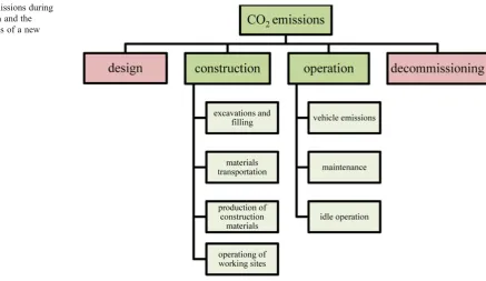
given project or activity over time, for the purpose of climate protection and the prevention of detrimental effects on human health. In civil engineering, it consists of four macro-phases over a long time-frame, namely design, construction, opera-tion and decommissioning (Fig. 1). Each of them must be taken into account in order to assess the overall scope.

The goal of such an analysis is to quantify a system’s incoming and outgoing CO2emissions in the various phases.

The CO2balance of a certain projectXin a given time frame is

positive if the overall CO2emissions produced (P) are lower

than the ones generated by the “do-nothing” scenario (N). Formally, this assumption can be expressed as follows:

BALCO2ðXÞ ¼NP ð1Þ

If BALCO2(X) >0, thenN > P: the CO2emissions of the

project are lower than those of the “do-nothing”scenario and hence there is a potential gain for the community. On the contrary, if BALCO2(X) <0, then the new project system

leads to a rise in emissions and its implementation should be discouraged.

2.1 CO2emissions for the construction of a new

transportation infrastructure

In the field of transportation engineering, the CO2balance

could be efficiently used in order to evaluate the environ-mental sustainability of a modified or newly-implemented traffic system or facility. In this last case, this method should take into account the indirect impact that such infrastruc-tures might have in terms of modal distribution of traffic.

To this end a comparison should be made between those scenarios following the building of the planned infrastruc-ture and others, in which no new construction is undertaken. Looking at the phases in Fig.1, from an operational view-point, the emissions resulting both from the design and the decommissioning phases are generally considered as negli-gible, since the former are of scarce relevance (0,03% in comparison with overall construction phase, [23]) and the latter concern interventions supposed to have a long life.

Also the construction phase seems to play a minor role in the process. In the calibration case chosen in this paper, it accounts only for about 4% overall (Fig.8)– smaller than the expected error of the methodology to calculate operation

emissions. The balance presented should however be ap-plied to a larger amount of cases to make this conclusion generalizable. For this reason, the impacts of the construc-tion phase are examined in short in secconstruc-tion2.2of this paper. In this framework, since construction is not to be consid-ered in the “do-nothing” scenario, the terms contained in formula (1) can be expressed as follows:

P¼CPþOP ð2Þ

N ¼ON ð3Þ

Where:

P are the total CO2emissions related to the project

analysed

CP are the total CO2emissions resulting from the

construction phase of the project

OP are the total CO2emissions resulting from the

operative phase of the project

N are the total CO2emissions related to the“do-nothing”

scenario

ON are the total CO2emissions resulting from the

operative phase of the“do-nothing”scenario.

The emissions resulting from the construction (C) and operation (O) phases may be further detailed in formulas (4) and (5) (Fig.2):

C¼CexþCtrþCprþCcn ð4Þ

O¼OvhþOupþOio ð5Þ

Where:

Cex are the CO2emissions produced by excavation and

filling operations

Ctr are the CO2emissions produced by materials

transportation operations

Cpr are the CO2emissions produced by construction

materials production operations

Ccn are the CO2emissions produced by operations to run

the working site

Ovh are the CO2emissions produced by vehicles

Oup are the CO2emissions produced by maintenance of

the infrastructure

Oio are the CO2emissions produced by idle operation.

Assuming 1 as the first year of operation of the new infrastructure andn as the last year to be included in the balance, lettingmbe the year in which construction of the infrastructure is accomplished (with m ≤ n), formulas (2) and (3) can be written as (6) and (7). The choice of the time horizon [1;n] must be well weighed, being based on several factors such as the expected life time of the infrastructure, the reliability of future forecasts etc.

P¼X

n

i¼1

Pi¼ Xm

j¼1

CPjþ Xn

i¼1

OPi ð6Þ

N¼X

n

i¼1

Ni¼ Xn

i¼1

OZi ð7Þ

Sections 2.2and 2.3 discuss in detail how the terms C andOcan be obtained.

2.2 Construction phase

In the construction phase analysis, the calculation of CO2

emissions is largely linked to the energy consumption, as anthropic CO2is released during all energy production and

transformation processes that involve combustion. The cal-culation method proposed is based on a bottom-up ap-proach: it takes into account the final energy consumption of the construction phase and the quantity of materials needed to build the infrastructure. Such data are converted into CO2emissions through appropriate factors.

Once the most significant elements of the entire construc-tion process are defined (Fig.2), these are then broken down into single operations in order to set up the calculation through simplifying assumptions, thus distinguishing relevant aspects from negligible ones.

The accuracy and validity of the results mostly depend on the quality of the data available. Therefore, it is crucial that the entire analysis be based on data as consistent and accurate as possible and capable of covering all the sectors considered. As regards the construction phase, the most useful instruments are the analysis of the available design documentation, an on-going dialogue with planners, direct observations and surveys. However, since the analysis is often carried out when the project is still in the assessment phase, there is limited knowledge of the actions and techniques used for construc-tion. To offset this situation, estimates need to be made based on analogy, on the study of the construction techni-ques, on the information collected from specialised firms and on scientific literature.

Once the final energy consumption for the single construc-tion operaconstruc-tions and the quantities of the materials used are obtained, these are converted into CO2emissions through the

following formula (8) for the construction phaseC:

C¼X

h

fhchþ X

k

qk8k ð8Þ

Where:

h is the specific energy source

fh is the final energy consumption obtained from the energy sourceh

χh indicates the CO2emission factors for the energy

sourceh Fig. 2 CO2emissions during

k is the type of material qk is the quantity of materialk

8k indicates the CO2emission factors for the materialk.

The emission factors can be estimated using regularly updated methods approved by international scientific bodies such as the Intergovernmental Panel for Climate Change [21]. Databases available in literature [16,35, 43] contain different values depending on the geographical area consid-ered and on the calculation method used. The conversion factors χh for energy consumption vary depending on whether the CO2emissions refer to the share of final energy

consumed or to the share of primary energy involved in the process.1Similarly, as regards the conversion factors8kfor the construction materials, these vary whether or not the emissions of the primary energy2are considered. Consisten-cy is essential when the emission factors to be used are selected: one should always specify whether the calculation is based on primary or final energy. Moreover, area-specific factors related to the geographical setting of the infrastructure should be preferred.

2.3 Operation phase

Operation-related CO2emissions must be calculated

consid-ering both options of maintaining of the status quo and modifying the existing transportation supply (e.g. by build-ing a new infrastructure). The key elements of the operation phase have already been identified as the number and type of vehicles, maintenance and idle operation (Fig.2).

One must also determine the territorial scale of reference based on the scope and the repercussions of the infrastruc-ture under consideration. These issues give rise to a series of methodological questions that are normally difficult to work out.

The scenario analysis offers an effective way to address the problem: after forecasting the most likely evolution over time, the pathways leading thereto are explored, as illustrated in Fig.3.

Estimated trends differ depending on the evolution of the considered parameters. Among these, the most im-portant ones concern the socio-economic conditions (population, GDP), social and technological development

and transportation policy (market organization, taxes and tariffs, infrastructure policies, adoption of requirements and bans). These factors determine the growth rates in the various scenarios. Therefore, future traffic flows can be quantified on the basis of historical data, provided that the latter are reliable and of good quality. The next step consists in calculating the CO2 emissions generated

by such scenarios. To do that, the amount of specific emissions per kilometre travelled is multiplied by the number of transiting vehicles according to the formula (9):

Ovh¼ Xn

i¼1

eividi

ð Þ ð9Þ

Where:

Ovh, 1, n have previously been defined

ei is the specific emission of vehicles and trains in the year considered

vi is the number of vehicles transiting in the year considered

di is the distance covered by vehiclevi.

The difficulty here lies in determining the trend of the specific traffic-related CO2emissions (ei), especially when the time horizon considered is quite extensive. Literature provides several methods for dealing with this issue (Cor-inair-IPCC [15], Copert [17] and Ecoinvent [43]). Infras [20] and Tremove [47] are two of the most commonly used software products to forecast future specific emissions on the basis of simple input data (country, region, network, period, fuel and vehicle type, vehicle technology and pol-lutant type) [20,47]. Differently from other methodologies that calculate emissions related to the covered distances or use only the tank-to-wheel emissions (i.e. Infras, Copert and Corinair), Tremove considers both the well-to-tank and tank-to-wheel emissions. Even if further researches in the field of specific emissions are required, CO2emission

mod-els generally provide more accurate results than other fore-casts on polluting gases [40], thus making the results more consistent.

3 The case-study: the Brenner base tunnel

The method previously described has been applied to the case study of the Brenner Base Tunnel (BBT), a 55 km long railway infrastructure that, once completed, will connect Austria (Innsbruck) with Italy (Fortezza/Franzensfeste).

The BBT belongs to the central sector of the TEN-T Corridor 1 that connects Berlin with Palermo with a 2,200 km long high-speed railway line. Due to the presence of the Alps, one of the most critical stretches of this line is 1

The CO2emission factorsχhfor final energy take into account the emissions related only to the energy quantified by the meter, whereas the emission factorsχhfor primary energy take into account also the share of emissions relating to the production, transportation of the energy source considered as well as the production, use and mainte-nance of the facilities used for its exploitation.

2_{The CO2emission factors8}

kfor primary energy (also referred to as

the Brenner corridor between Kufstein, a town close to the Austrian-German border, and Verona (Fig.4).

The Brenner corridor is commonly divided into three sections:

– Northern access route (Munich – Kufstein, Kufstein– Kundl, Kundl–Baumkirchen);

– Brenner Base Tunnel (Innsbruck–Fortezza/Franzensfeste) with the Innsbruck bypass;

– Southern access route (Fortezza/Franzensfeste – Ponte Gardena/Waidbruck, Bolzano/Bozen bypass, Trento bypass, Verona approach).

The entire line will be upgraded in different phases: the works are currently at a more advanced stage in the Northern access route than in the Southern one.

The BBT represents the central sector that links the two parts of the line. The construction phase of the main tunnels

began in April 2011 and is planned to be completed by 2022, barring any setbacks.

In calculating the CO2emissions of the construction and

operation phases, two different spatial scopes were used. While construction-related emissions refer to the realization of the infrastructure (i.e. the 55 km long tunnel: paragraph 3.1), operation-related emissions consider the transnational impact of the tunnel and its effects on the entire line. Therefore, the traffic scenarios (paragraph 3.2) refer to the line as a whole, including all Italian and Austrian sectors between Kufstein and Verona.

3.1 Construction phase

The BBT infrastructure is schematized in Fig.5.

Main tubes, exploratory tunnels, side tunnels, multi-purpose areas, lateral access and the interconnections with Fig. 3 Outline of the scenario

method

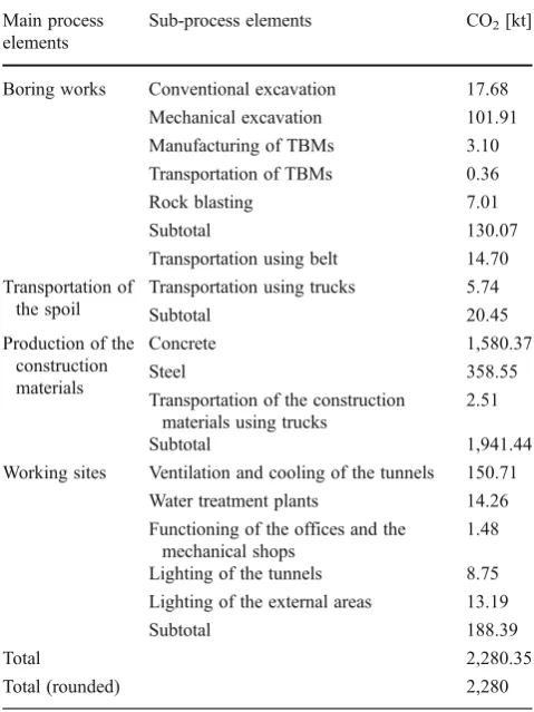
Fortezza and the Innsbruck bypass are the components considered during the calculation phase. In the following analysis, most of the data and values derive from the final design drawn up by BBT SE [4]. Figure 2 lists the main process elements that should be taken into account in the CO2 balance of the construction of a tunnel. The largest

energy consumption and consequently the CO2 emission

peak are normally generated during the excavation phase, the transportation of the spoil to the deposits, the production of the materials used to coat the tunnels and the running of the working sites [33]. These elements have been specified into the sub-process elements listed in Table1.

In the case of the BBT, the tunnel is excavated using the conventional method with excavators and rock blasting, and the mechanical method with the Tunnel Boring Machine

(TBM). The method to be used is chosen on the basis of the geological and geotechnical surveys and the cross section, as well as on the length and gradient of the tunnel section to be built. The calculation estimates mainly the energy consump-tion of the machines used. In the convenconsump-tional excavaconsump-tion, also the CO2 released during rock blasting is factored in.

Likewise, in the mechanical excavation, the CO2emissions

resulting from the production of TBMs and their transportation from the production to the working sites are included.

Table 1 Main process elements of the analysis. Source: [33], elaborated

Main process elements Sub-process elements

Boring works Conventional excavation Mechanical excavation Manufacturing of TBMs Transportation of TBMs Rock blasting

Transportation of the spoil

Transportation using belt Transportation using trucks Production of the

construction materials

Concrete Steel

Transportation of the construction materials using trucks

Working sites Ventilation and the cooling of the tunnels Water treatment plants

Functioning of the offices and the mechanic shops

Lighting of the tunnels Lighting of the external areas Fig. 5 Overview of the

Brenner Base Tunnel system. Source: [5], elaborated

Table 2 CO2emissions in the construction phase of the BBT

Main process elements

Sub-process elements CO2[kt]

Boring works Conventional excavation 17.68 Mechanical excavation 101.91 Manufacturing of TBMs 3.10 Transportation of TBMs 0.36

Rock blasting 7.01

Subtotal 130.07

Transportation using belt 14.70 Transportation of

the spoil

Transportation using trucks 5.74

Subtotal 20.45

Production of the construction materials

Concrete 1,580.37

Steel 358.55

Transportation of the construction materials using trucks

2.51

Subtotal 1,941.44

Working sites Ventilation and cooling of the tunnels 150.71 Water treatment plants 14.26 Functioning of the offices and the

mechanical shops

1.48

Lighting of the tunnels 8.75 Lighting of the external areas 13.19

Subtotal 188.39

Total 2,280.35

The materials used to build the infrastructure are mainly cement and steel, with the latter used mostly for anchoring, building bridges and the production of rein-forced concrete. Emissions due to the use of plastic material for the piping and other finishing materials are assumed to be negligible.

The transportation of the construction materials and the spoil to the deposits is then considered: a distinction

is made between belt and truck method on account of the different energy consumption of the two forms of transportation.

The CO2 emissions related to the construction site

in-clude those generated by the tunnel ventilation and cooling systems, the water treatment plants, the mechanical shops and offices. Finally, the contribution of the lighting of the tunnels and external areas are considered.

Table 3 Measures to discourage the use of road transportation adopted in“minimum”,“trend”and“consensus”scenarios. Source: [32], elaborated

Minimum Trend Consensus

Measures to discourage the use of road transportation

Road costs per km

Current costs Current costs +30% in comparison with other scenarios

Road tolls (passengers)

No tolls related to the covered distance; no urban tolls

No tolls related to the covered distance; no urban tolls

No tolls related to the covered distance. Introduction of urban tolls. General costs +15% in comparison with other scenarios

Road costs (freight)

Highway tolls under infrastructural costs up to 2015

Highway tolls at the same level as infrastructural costs up to 2015

Highway tolls higher than infrastructural costs (+15% in comparison with trend scenario); harmonization of tolls in all the Alpine arc Road traffic

ban

No ban along Brenner highway, maintenance of Sunday and nocturnal bans, use of dosage systems

No ban along Brenner highway, maintenance of Sunday and nocturnal bans, use of dosage systems

Implementation of social and security prescriptions, no ban along Brenner highway, maintenance of Sunday and nocturnal bans, use of dosage systems

Speed-limits No changes No changes More controls, reductions of a good 8% Tax on mineral

oil

Uniform tax rate on all the EU countries based on present value

Uniform tax rate on all the EU countries based on present value

Uniform tax rate on all the EU countries higher than present value; introduction of an eco-tax Enforcement of

roads

Enforcement of highways (but not along Alps)

Enforcement of highways (but not along Alps)

Investments only for national programs or for TEN-T to reduce bottlenecks

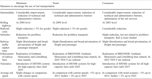
Table 4 Measures to encourage the use of rail transportation adopted in“minimum”,“trend”and“consensus”scenarios. Source: [32], elaborated

Minimum Trend Consensus

Measures to encourage the use of rail transportation

Intermodality Considerable improvement, reduction of technical and administrative barriers

Considerable improvement, reduction of technical and administrative barriers

Considerable improvement, reduction of technical and administrative barriers, optimization of the rail services Rolling

highway

At 2004 level At 2004 level At 2003 level

Railroad costs

Slight reduction (−5% for goods) Slight reduction (−5% for goods) Considerable reduction

Subsidies Reduction for profitless transports

Reduction for profitless transports Slight reduction, but not related to profitless transports. Rail is more funded

Railway traffic market rules

Slight liberalization and broad privatization of freight and passenger transport

Slight liberalization and broad privatization of freight and passenger

Slight liberalization and broad privatization of freight and passenger

Enforcement of railway lines

Realization of Gotthard, Moncenisio and Lötschberg base tunnels

Realization of BRENNER, Gotthard, Moncenisio and Lötschberg base tunnels. In 2025 TEN-T are realized

Realization of BRENNER, Gotthard, Moncenisio and Lötschberg base tunnels. In 2025 TEN-T are realized

Telematics Introduction of ERTMS systems for high-capacity lines until 2025

Introduction of ERTMS systems for high-capacity lines until 2025

Introduction of ERTMS systems for all high-capacity lines until 2015

Average rail speed

Slight changes in comparison with current speed

In comparison with current speeds: +3% up to 2015, further + 2% up to 2025

After calculating the energy consumption [33], values are converted into CO2 emissions by applying the following

emission factorsXh, expressed in kg CO2/kWh:

Xg00.202 for energy obtained from natural gas [21];

Xd00.267 for energy obtained from diesel oil [21];

Xel,IT00.435 for electricity generated in Italy [44];

Xel,A00.216 for electricity generated in Austria [44].

The emissions resulting from the combustion of crude oil derivatives are calculated by referring to the guidelines provided by the IPCC [21], while the calculation of the emissions deriving from electricity are based on Terna’s studies [44]. Since about 60% of the infrastructure is located in Austria and the remaining 40% is in Italy, the combined average of the energy mix of both countries was considered. Specific emission factors (8k) are then provided for the construction materials. The data about concrete are provided by BBT SE, while the data about steel are provided by the Munich-based FFE research centre [16], as specific values are not available for Italy and Austria. Emission factors are expressed in kg CO2/t:

8steel, structural01.980 [16];

8steel, machines01.449 [16];

8portland cement0622;

8pozzolanic cement0576.

Both factors (Xhand8k) estimate the CO2emissions

result-ing from the consumption of primary energy, takresult-ing into account the emissions related to the entire process and not only to the final energy, as described in footnotes 1 and 2.

Energy consumption and material quantities are con-verted into CO2emissions using CO2emission factors

(for-mula 8). The total amount of CO2associated with the BBT

construction phase is about 2,280 kt (Table2).

3.2 Operation phase

Recalling Fig.2, emissions in the operation phase arise from vehicles, maintenance and idle operation. The last two fac-tors are not calculated as their overall emissions are consid-ered negligible in comparison with the vehicle emissions.

The calculation is based on a study by ProgTrans [37], which analyses the evolution of transportation along the Brenner axis (i.e. the Brenner rail line and the Brenner highway) up to 2030 in terms of average annual variations in freight and passenger traffic, by the development of six different scenarios.

3.2.1 The future traffic demand

In order to determine the future traffic demand and to provide the possible growth rates, ProgTrans adopts a classical four-stage model [30]. An area which includes 37 countries (all EU countries – except for Malta and Cyprus – , Switzerland, Norway and South-East European countries) is analysed: most of them are considered on NUTS 0-level, except for Austria, Germany, Italy, France, Netherlands, Belgium and Switzerland (NUTS 2) and the Alpine area (NUTS 3).

The traffic generation is calculated depending on five main parameters: socioeconomic tendencies, technological development, transportation policies, social changes (for passengers) and development of transportation economy and logistics (for goods).3

3_{In detail, three main fields are considered among the socioeconomic} tendencies: the division in different classes of age of the overall population, the gross domestic product and the import/export business. The social aspects involve mostly the life style of the families and its changes in the next years. The main differences among the hypothesis introduced are related to the transportation field: different market regulations, fiscal and infrastructural policies, prescriptions and bans. Table 5 Overview of results of the mean annual variations of traffic along the Brenner axis. Source: [37], elaborated

Brenner growth rates - Freight Brenner growth rates - Passengers

Minimum Trend Consensus Minimum Trend Consensus

Road Rail Road Rail Road Rail Road Rail Road Rail Road Rail

2009–2015 1.9% 3.1% 1.9% 3.1% 0.1% 3.1% 1.2% 3.1% 1.2% 3.1% 0.7% 3.1% 2016–2020 1.5% 2.1% 1.5% 7.7% −0.1% 8.6% 1.9% 2.1% 1.9% 4.8% 2.2% 5.3% 2021–2025 1.5% 2.1% 1.3% 6.9% −0.6% 7.4% 1.9% 2.1% 1.9% 4.5% 2.2% 5.0% 2026–2030 1.0% 1.2% 1.4% 1.9% 0.0% 2.3% 1.5% 1.7% 1.4% 3.8% 1.5% 4.2% 2031–2035 1.0% 1.2% 1.4% 1.9% 0.0% 2.3% 1.5% 1.7% 1.4% 3.8% 1.5% 4.2%

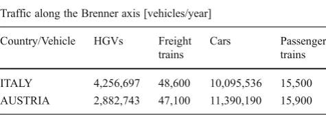
Table 6 Traffic demand along the Brenner axis in 2008. Sources: [1, 29], elaborated

Traffic along the Brenner axis [vehicles/year]

Country/Vehicle HGVs Freight trains

Cars Passenger trains

The distribution is provided by the use of an origin– destination matrix, which includes 296 traffic cells. The modal choice is based on the generalized costs, which include both the distance costs and the travel costs. The former are meant as the sum of the costs necessary to transport a freight train or a HGV (freight transportation) or a person (passenger transportation) for a kilometre; the latter include fixed costs for the exercise of a transportation system (HGVs, freight trains, passenger trains or cars), energy and tracing costs and tolls.4

Finally, the route assignment is developed for both road and rail traffics. The former is obtained through TRIBUT [2], a capacity restraint method based on a bicriterion path search algorithm which includes times and costs as param-eters. The latter is calculated through a procedure which takes into account the aggregate travel time of four different systems [37]: three of them are related to the passenger transportation (namely high speed, intercity/eurocity and regional trains), while the fourth is linked with good trans-portation (freight trains).

At the end of this method, six different scenarios are determined. Only three of them are included in the balance, as the assumptions of the other three are deemed either unlikely (two of them consider the new Gotthard Base Tunnel not in use – even though it is currently at an advanced stage of construction) or incom-plete (forecasts considered freight traffic only). Three scenarios are therefore taken into account, in this paper

called“minimum”,“trend”and“consensus”, whose main points are shown in Tables 3 and 4.

The“minimum”scenario coincides with the maintenance of the do-nothing, i.e. the BBT is not built, while both the

“trend” and “consensus” scenarios are based on the con-struction of the tunnel.

The difference between these last two scenarios lies in the transportation policies. The continuation of the trend of the last decade is considered in the “trend”scenario, namely a market liberalisation that boosts road traffic. This policy should encourage the development of rail transportation. At the same time, the absence of measures to discourage the use of road vehicles should cause also a demand increase of HGVs and cars. It follows that an higher amount of overall traffic is generated, if compared with the two other scenarios.

The latter (“consensus” scenario) foresees a series of actions to foster the growth of railway traffic and encourage the simultaneous reduction of road traffic. The following measures are introduced in order to reach the complete internalization of external costs: in the field of tax policy, the increase of tolls (Austrian tolls are assumed to reach the Swiss ones) for all the types of vehicles and the funding of the railway mode. The introduction of an eco-tax for mineral oil and the reduction of transportation subsidies are also forecasted. Related to the infrastructural policy, the im-provement of the high-speed rail line (with subsequent reduction of travel time), the development of the rolling highway and the modernization of the materials are sched-uled. In relation to the road empowerment, only the most critic bottlenecks are solved (no further construction of road segments between the Alpine highways).

Finally, a scenario which includes only restriction to the circulation of the vehicles is considered unrealistic and therefore not analysed here: it foresees only constrictions to the free circulation, thus being against the important principle of “social equity” promoted by the EU in the development of its transportation policy.

Originally up to 2030, the forecasts were extended to 2035, thus determining a time horizon for the Brenner Base Tunnel of 25 years (Table 5). The values shown are mean annual growth rates.

As above mentioned, the growth of rail traffic (both for passengers and goods) in the “consensus” and “trend” 4

In order to ease the comprehension of the modal choice, the values of the costs in the scenarios analyzed in this article are here provided. In

“trend”scenario, the values are as follows: for the goods, the distance costs are 34.10€for every freight train and kilometre, reduced to 31.90

€from 2015, and 0.57€for every HGV; time costs are, respectively, 68.20 and 34.10€. This value considers a type-train of 420 t up to 2015 and of 500 t train from 2015; HGVs are divided in 10 classes, consid-ering the different goods transported; the capacity is supposed stable up to 2035. For the passengers, the distance costs are currently 0.085€for every train passenger and 0.10€for every car passenger; time costs are 9.15€both for rail and road. In“consensus”scenario, the values are as follows: for the goods, the distance costs are the same as in“trend” scenario for rail; only the capacity of the type freight train is supposed to change, being 425 t up to 2015, 550 t in 2015 and 605 t in 2025. For road freight transportation, costs increase to 0.68€ for every HGV from 2015 to 0.75€from 2025. The capacity as well as the time costs are the same as in the“trend”scenario.

Table 7 Traffic along the Brenner axis. Forecast for 2035 [vehicles/year]. Source: [38]; elaborated

Italy Austria

Scenario HGVs Freight trains Cars Pax trains HGVs Freight trains Cars Pax trains

scenarios is due to the introduction of the BBT and the high speed rail line. They allow the use of new tracks, thus imple-menting the overall railway capacity and rationalizing the line already existing. The growth rate of freight rail transportation is higher than the passenger one. This result can be explained by the nature of BBT, which is supposed to introduce about 400 new trains per day: according to the traffic simulations developed by BBT SE, about 75% of them will be introduced for freight transportation and the leftover for passengers [3]. This is the reason for which the expected growth rates of rail freight transportation are much higher than passengers’. Indi-rectly, it justifies also the difference between road passenger traffic of“consensus”and“trend”scenarios.

The number of vehicles circulating up to 2035 is then obtained by multiplying the rates listed above by the histor-ical data [1,29; Table6]. The analysis considers both freight and passenger traffic on road and rail. By way of example, Table7shows the data for 2035 alone.

3.2.2 The future specific emissions

The Infras Handbook and the Tremove software applica-tions are used to determine the average specific emissions for road and railway traffic respectively [20, 47]. Both software applications provide the trend of the specific emissions over five-year periods (Table 8).

Tremove software includes the following parameters: country, region, network, period, fuel type, vehicle type, vehicle technology, pollutant type. Each of them requires a choice among several possibilities: for example, referring to the vehicle technology, the choice is among passenger train, bus, car, heavy duty truck >32 t, heavy duty truck 6–32 t, heavy duty truck 3.5–7.5 t, heavy duty truck 7.5–16 t, light duty truck, moped, motorcycle, van, plane, freight train, inland ship, metro/tram [24].

Infras handbook considers the following parameters: coun-try, vehicle type, polluting gases, year, fleet composition, Table 8 Calculation of the trend

in CO2emissions for road traf-fic. Source: [20,47], elaborated

Road Rail

Year Automobiles [g/veh km] Trucks [g/veh km] Pax trains [g/veh km] Freight trains [g/veh km]

1990 186 855 5,890 14,860

1995 180 796 5,730 13,830

2000 174 720 5,440 12,670

2005 167 718 5,200 10,960

2010 160 717 4,970 9,260

2015 155 710 4,930 8,970

2020 151 703 4,900 8,680

2025 143 680 4,850 8,290

2030 137 671 4,770 7,820

2035 131 663 4,700 7,400

Table 9 CO2 emissions produced by road and railway traffic. Kufstein-Verona section. Source: [38], elaborated

Minimum Trend Consensus Year CO2emissions

(kt)

CO2emissions

(kt)

CO2emissions

(kt)

2010 1,535 1,535 1,500

2011 1,555 1,555 1,502

2012 1,581 1,581 1,510

2013 1,608 1,608 1,518

2014 1,635 1,635 1,526

2015 1,663 1,663 1,534

2016 1,690 1,696 1,542

2017 1,715 1,726 1,565

2018 1,741 1,762 1,589

2019 1,767 1,801 1,615

2020 1,793 1,840 1,643

2021 1,805 1,866 1,659

2022 1,817 1,889 1,670

2023 1,829 1,913 1,681

2024 1,840 1,937 1,695

2025 1,852 1,963 1,709

2026 1,873 1,998 1,733

2027 1,885 2,017 1,740

2028 1,897 2,036 1,748

2029 1,909 2,055 1,755

2030 1,921 2,074 1,763

2031 1,934 2,094 1,772

2032 1,946 2,114 1,780

2033 1,959 2,135 1,788

2034 1,972 2,155 1,797

2035 1,984 2,176 1,805

Total 46,706 48,822 43,139 Total

(rounded)

network, level of service, speed limit, parameters for hot emissions factors and cold start access [46]. The evaluation of the specific emissions is based on the type-vehicle. Two trains (one for each railway line) are considered for the freight transportation: the one going through the existing line has two locomotives, a max speed of 100 km/h, an overall weight of 1,200 t. The other one has only one locomotive and same attributes. The train for passengers is an Intercity express type 1 (length: 200 m, average number of passengers: 400; gross weight: 435 t). Data are extracted from an exercise document of the Monaco-Verona line, provided by BBT SE.

For the road, the standard vehicle for goods is an HGV of 32 t. Average speed is 80 km/h and it is powered by diesel. The class of the engine depends on the year considered. The

standard vehicle for passengers is a car with an engine of 1,600 cc. Maximum speed is 130 km/h and it is powered by diesel. Also in this case, the class of the engine depends on the year considered.

The constant decreasing values presented in Table8are due to the progress in the technology field, which grants the development of more efficient engines and vehicles.

3.2.3 The future overall emissions

The total emissions in the various scenarios were obtained for the years 2010–2035 by multiplying the number of vehicles by the mean specific emissions and by the distances travelled (formula 9).

+200 kt

-180 kt

Fig. 6 CO2emissions in the various scenarios: yearly variations. Source: [38], elaborated

Distances were calculated usingwww.viamichelin.it for road,http://pedaggio2004.rfi.it for the Italian sector of the railway line andwww.oebb.at for the Austrian one. From these calculations, the road distance for the Italian rail and road stretches (Verona-Brenner) are, respectively, 220 and 226 km; for the Austrian one (Brenner-Kufstein), respectively 111 and 106.

As soon as all these data are known it is possible to determine the yearly overall CO2 emissions by using the

method described in section2(Table9).

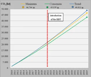
Table 9 shows that the overall lowest CO2 emissions

(about 43,150 kt) are forecasted in the“consensus”scenario, followed by the “minimum” and “trend” scenarios, with about 46,700 kt and 48,800 kt respectively.

As the year of reference increases, the difference in the emissions between the scenario without tunnel and the two scenarios with tunnel increases as well. In 2035, the“ con-sensus”scenario produces about 180 kt CO2emissions less

than the “minimum” scenario, while the “trend” scenario implies an increase in emissions of about 200 kt (Fig.6).

Three aspects need here a further explanation.

First, although the BBT is expected to be working only by 2022, the variations in CO2emissions between the“

con-sensus”scenario on the one side, and the“trend”and“ min-imum” scenarios on the other, are already visible starting from 2010 on. This is mainly due to a supposed different behaviour of freight operators: ProgTrans forecasts [37] consider the traffic support policy (as described above) to be strictly linked to the opening of the tunnel. Some of these measures are supposed to be put into force already in 2010 in order to obtain a gradual but constant shift from road to rail (“consensus”scenario) or a gradual growth of traffic rail (“trend”scenario). Both these conditions are supposed to be fully realized in the first operation year of the tunnel (be-lieved 2022). In this year, at these traffic growth rates the

current Brenner railway line by itself would not have the capacity to serve the demand of neither of these two scenarios.

Second, “minimum” and “trend” scenarios show the same rise between 2010 and 2015. This should be consid-ered an expected result, as both call for the same traffic growth forecasts (Table5).

Third, the overall trend in the “consensus” and “ mini-mum”scenarios seems to have a similar shape in the years 2016–2035 (Fig. 6). This is mostly an undesired visual impression: a rough data comparison can confirm this state-ment.5This means that the two curves are divergent and the difference in CO2emissions is progressively increasing.

The overall CO2 emissions for the years 2010–2035

deriving from the operation phase (Fig. 7) confirm these considerations, showing how the main differences in the three scenarios are broader after the opening of the BBT (2022).

3.3 Result comparison

Table 9 and Fig. 8 show the impacts of the BBT on CO2

emissions, which are supposed to be about 46,700 kt in the do-nothing case (“minimum”scenario). If the tunnel is real-ized, future emissions will depend on the policies adopted. If the support measures for the railway are adequate, the road traffic is likely to decrease and the overall CO2emissions are

expected to be lower than in the“minimum”scenario. They will amount to about 45,400 kt, equal to the sum of the emissions resulting from the construction of the tunnel

5_{In 2021, CO2emissions are supposed to be 1,696 kt for the“trend”} and 1,542 for the “consensus”scenario – it makes a difference of 144 kt. In 2035 this difference rises up to 371 kt–2,176 kt in“trend” and 1,805 kt in“consensus”scenarios.

(2,280 kt) and from the “consensus” scenario (about 43,150 kt). Therefore, recalling formula (1), BALCO2(BBT) >0.

On the other hand, if policies adopted continue the cur-rent trend, rail and especially road traffic will further in-crease. As a consequence, also emissions are expected to grow and reach about 51,100 kt, which is the sum of the emissions resulting from the tunnel construction (2,280 kt) and the “trend” scenario (about 48,800 kt). In this case BALCO2(BBT) <0.

Figure8shows that the construction of the BBT does not necessarily imply a reduction in CO2emissions; indeed, the

tunnel might lead to a considerable increase due to the traffic demand growth, as evidenced by the“trend”scenario, which yielded 4,400 kt CO2more than the“minimum”one.

Only if duly supported by a correct policy favouring rail-ways the tunnel will help cut CO2emissions (“consensus”

scenario,−1,300 kt).

As far as “minimum” and “consensus” scenario are concerned, the overall CO2emissions are cut only by about

3%. This value could be considered disappointing if taken by itself. It should rather be taken into account in connection with its relative traffic demand: in the period 2010–2035, a 29% emission increase in the“minimum”scenario (1,535– 1,984 kt) is for instance accompanied from a 75% freight railway increase (51,660–85,033 trains).

As well, in“consensus”scenario the emissions are sup-posed to grow from 1,500 kt (in 2010) to 1,805 kt (in 2035, +20%), but the overall amount of freight trains circulating should treble (51,660 in 2010 and 164,345 in 2035) and is almost double than in“minimum”scenario. Similar consid-erations can be stated for the other traffic modes analysed.

4 Values and faults of the method described

The method described in this paper was conceived to relate carbon dioxide emissions to modifications in the transpor-tation supply. It can be used either as an independent tool or within a Multi-Criteria Evaluation.

In both cases, further research is required on the interac-tion between the effects of the simplificainterac-tions adopted and the accuracy of the model results. Particularly, as the impact of the emissions depends from a certain number of key variables (here identified with the estimation of overall road traffic, its modal shift, and the technological improvement of the vehicles circulating), the extension of the time frame at stake makes hard quantifying model uncertainty, thus denying an important information for decision-making.

If the construction of a new infrastructure is included in the process, then the considerable width of the time frame cannot be avoided and should be retained as a model feature. This obviously makes the estimation of the evolution of the key-variables not reliable onex-postevaluations. As in any

forecast, however, the containment of the referential period makes the control of the results easier.

The Brenner Base Tunnel was here reported as a case study. The main benefit from the construction of this infrastructure should be considered the time reduction for the connections between the cities along the stretch of the Munich-Verona high speed line at a lower average pollution rate. In mere terms of carbon dioxide, however, the results reveal that the effect of the tunnel may be strengthened if added to an adequate policy in favour of the railway and that the amounts of CO2produced

should not be considered by themselves but in connection with their relative travel demand.

Though it probably needs to be further refined and some of its limitations need to be better understood, the necessary changes having been made, the method described herein is considered to be fully applicable throughout transportation planning. In fact, it may cover all the cases of implementation of new systems, changes in existing systems, or construction of new infrastructures. Its hypotheses are sufficiently flexible, and the number of equations and assumptions used was kept as small as possible. The model only requires that input data be adequately detailed in terms of vehicle shares, fuel con-sumption per vehicle and distance travelled–a result that can be achieved from planners, decision-makers and stakeholders by allocating adequate resources for data collection.

Acknowledgement This research was developed at the European Academy in Bolzano and partly funded under grant No. D0363 by both the European Academy of Bolzano and BBT public limited company. A noticeable amount of data and values used in the article was provided by BBT-SE, whose support is here gratefully acknowledged.

Open Access This article is distributed under the terms of the Creative Commons Attribution License which permits any use, distribution and reproduction in any medium, provided the original author(s) and source are credited.

References

1. Aiscat (2009) Aiscat informazioni. Quarterly Report Online at: http://www.aiscat.it/pubblicazioni/downloads/trim3-4-09.pdf [01-02-2011]

2. Barbier-Saint-Hilaire F et al (1999) TRIBUT–a Bicriterion ap-proach for equilibrium assignment. PTV AG, Karlsruhe

3. BBT SE (2008a) Technische Projektaufbereitung - Elaborazione tecnica del progetto. Online at: http://www.bmvit.gv.at/verkehr/ eisenbahn/verfahren/bbt/bbt3a/dokumente/D0118-02368.pdf [26.05.2011]

4. BBT SE (2008b) Potenziamento asse ferroviario Monaco–Verona. Galleria di Base del Brennero. Progetto definitivo. Relazione tecnica [29-03-2008]

5. BBT SE (2009) Il sistema della Galleria di Base del Brennero. Online at:http://www.bbt-se.com/index.php?option0com_content &task0view&id0111&Itemid0223&lang0it[02-03-2011] 6. Black WR (2010) Sustainable transportation: issues and solutions.

7. Bollen J, van der Zwaan B, Eerens HC, Brink C (2009) Local air pollution and global climate change: a combined cost-benefit analy-sis. Resour Energy Econom 31:161–181

8. Booz Allen Hamilton Ltd (2007) Estimated carbon impact of a new north-south line. Research report. Online at:http://webarchive. nationalarchives.gov.uk/+/http:/www.dft.gov.uk/pgr/rail/ researchtech/research/newline/carbonimpact.pdf[10-10-2011] 9. Börjesson PII (1996) Emissions of CO2from biomass production

and transportation in agriculture and forestry. Energ Convers Manag 37(6–8):1235–1240

10. Bundesministerium für Verkehr, Innovation und Technologie (BMVIT) (2008) Lageplan Gesamtstrecke der Achse München-Verona

11. Campos Gouvea VB, Ramos RAR, de Miranda D, Correia S (2009) Multi criteria analysis procedure for sustainable mobility evaluation in urban areas. J Adv Transp 43(4):371–390

12. Contaldi R, Ilacqua M (2003) Analisi dei fattori di emissione di CO2dal settore dei trasporti, APAT report 28/2003

13. de Carvalho Macedoa I (1998) Greenhouse gas emissions and energy balances in bio-ethanol production and utilization in Brazil (1996). Biomass Bioenergy 14(1):77–81

14. European Environment Agency (EEA) (2010) The European en-vironment state and outlook 2010 synthesis. Copenaghen, 2010. Online at: http://www.eea.europa.eu/soer/synthesis/synthesis [13-10-2011]

15. EMEP/EEA (2009) Air pollutant emission inventory guidebook. Online at: http://www.eea.europa.eu/publications/emep-eea-emis sion-inventory-guidebook-2009[01-03-2011]

16. Forschungsstelle für Energiewirtschaft (FFE) (2009) Online at: http://www.ffe.de/taetigkeitsfelder/ganzheitliche-energie-emis sions-und-kostenanalysen/200-gabie-ganzheitliche-bilanzierung-von-prozessen-und-produkten[01-12-2009]

17. Gkatzoflias D, Ntziachristos L, Samaras Z (2007) Computer programme to calculate emissions from road transport - users manual. European topic centre on air and climate change. Online at:http://www.emisia.com/copert/[01-03-2011]

18. Hansen J, Sato M, Kharecha P, Beerling D, Masson-Delmotte V, Pagani M, Raymo Maureen, Royer DL, Zachos JC (2008) Target atmospheric CO2: where should humanity aim? Open Atmos Sci J 2:pp 217–231. Online at: http://arxiv.org/ftp/arxiv/papers/0804/ 0804.1126.pdf[13-10-2011]

19. Hidalgo I, Szabo L, Ciscar JC, Soria A (2005) Technological prospects and CO2emission trading analyses in the iron and steel industry: a global model. Energy 30(5):583–610

20. INFRAS (2010) The Handbook Emission Factors for Road Transport (HBEFA).http://www.hbefa.net[15-01-2010]

21. Intergovernmental Panel on Climate Change (IPCC) (2006) 2006 IPCC guidelines for national greenhouse gas inventories, prepared by the national greenhouse gas inventories programme. In: Eggleston HS, Buendia L, Miwa K, et al. (eds) Published: IGES, Japan 22. Intergovernmental Panel on Climate Change (IPCC) (2007)

Con-tribution of working groups I, II and III to the fourth assessment report of the intergovernmental panel on climate change. Climate Change 2007: Synthesis Report. Geneva

23. Italferr (2010) Rapporto di sintesi sulla emissione (rimozione) della CO2. Progetto Definitivo “Potenziamento linea Rho-Arona: tratta Rho– Gallarate”. Online at:http://www.italferr.it/cms-file/allegati/ italferr/Rapporto_di_sintesi_Gallarate_Rho_rev2.pdf[01-02-2011] 24. Keller M (2010) Handbook emission factors for road transport 3.1.

Quick reference. Infras, Bern

25. Kiese R, Butterbach-Bahl K (2002) N2O and CO2emissions from three different tropical forest sites in the wet tropics of Queensland, Australia. Soil Biol Biochem 34(7):975–987

26. Köne AC, Büke T (2010) Forecasting of CO2emissions from fuel combustion using trend analysis. Renew Sustain Energ Rev 14 (9):2906–2915

27. Konidari P, Mavrakis D (2007) A multi-criteria evaluation method for climate change mitigation policy instruments. Energy Policy 35–12:6235–6257

28. Kouloumpis V, Kouikoglou VS, Phillis YA (2008) Sustainability assessment of nations and related decision making using fuzzy logic. IEEE Syst J 2(2):224–236

29. Land Tirol (2009) Verkehrsentwicklung in Tirol 08/09. Online at: http://www.tirol.gv.at/fileadmin/www.tirol.gv.at/themen/verkehr/ verkehrsplanung/VDE/ta_automatische_zaehlungen0809.pdf [01-02-2011]

30. McNally MG (2008) The four step model. Center for activity systems analysis. Institute of Transportation Studies, UC Irvine 31. Network rail (2009) Comparing environmental impact of

conven-tional and high speed rail. Online at:http://www.networkrail.co.uk/ documents/ About%20us/New%20Lines%20Progr amme/ 5878_Comparing%20environmental%20impact%20of%20con ventional%20and%20high%20speed%20rail.pdf[01-02-2011] 32. Nocera S, Cavallaro F (2011) Policy effectiveness for containing

CO2emissions in transportation. Proced Soc Behav Sci 20:703– 713

33. Nocera S, Maino F, Wagner M (2010) Calculation of the energy consumption for the construction of a railway tunnel. In: Martin U. et al. (eds) Network for Mobility 2010 (Proceedings of the 5th International Symposium). Stuttgart: FOVUS, 2010-09-30 34. Nordhaus W (2007) The challenge of global warming: economic

models and environmental policy. Online at:http://nordhaus.econ. yale.edu/dice_mss_072407_all.pdf[13-10-2011]

35. Öko-Institute e V (2011) GEMIS - global emission model for integrated systems. Online:http://www.oeko.de/service/gemis/en/ [01-03-2011]

36. Phillis YA, Grigoroudis E, Kouikoglou VS (2011) Sustainabil-ity ranking and improvement of countries. Ecol Econ 70(3): 542–553

37. ProgTrans AG (2007) Aggiornamento della previsione sul traffico merci e passeggeri per il Brennero al 2015 e 2025. Research Report, Zürich, Switzerland. Online at: http://www.bmvit.gv.at/verkehr/ eisenbahn/verfahren/bbt/uvp/progtrans_prognose.pdf[13.10.2011] 38. Ruffini FV, Maino F, Nocera S (2010) Sostenibilità del tunnel di

Base del Brennero in rapporto alle emissioni di CO2. Research Report, Bolzano, Italy

39. Sinha KC, Labi S (2007) Transportation decision making - principles of project evaluation and programming. Wiley, New York 40. Smit R, Ntziachristo L, Boulter P (2010) Validation of road vehicle

and traffic emission models. A review and meta-analysis. Atmos Environ pp 2943–2953

41. Song C (2006) Global challenges and strategies for control, con-version and utilization of CO2for sustainable development involv-ing energy, catalysis, adsorption and chemical processinvolv-ing. Catal Today 115:2–32

42. Stern N (2006) Stern review on the economics of climate change, UK Treasury. Online at: http://webarchive.nationalarchives.gov.uk/+/ http://www.hmtreasury.gov.uk/stern_review_report.htm[22-06-2011] 43. Swiss Center for Life Cycle Inventories (2011) Ecoinvent

data-base. Online at:http://ecoinvent.ch/[01-03-2011]

44. Terna (2009) Dati statistici sull’energia elettrica in Italia. Confronti internazionali. Online:http://www.terna.it/LinkClick.aspx?filetick et0PgmBzvheblE%3d&tabid0418&mid02501[01-03-2011] 45. Thornes JE (1992) The impact of weather and climate on transport

in the U.K. progress. Phys Geogr 16:187–208

46. Transport & Mobility Leuven (2007) TREMOVE model descrip-tion. Online at: http://www.tremove.org/documentation/TREMO VE_Short_Description.pdf[21.06.2011]

48. Transportation Research Board (TRB) (2008) Potential impacts of climate change on U.S. Transportation. Special Report 290. National Research Council, Transportation Research Board, Washington, DC

49. Tuchschmid M (2009) Carbon footprint of high-speeds railway in-frastructure (Pre-study). Methodology and application of high speed railway operation of European railways. Online at:http://uic.asso.fr/ IMG/pdf/carbon_footprint_of_high_speed_rail_infrastructure _pre-study.pdf[01-02-2011]

50. Turkenburg W (1997) Sustainable development, climate change, and carbon dioxide removal. Energ Convers Manag 38(1):S3– S12

51. UN, United Nations (1998) Kyoto protocol to the United Nations framework convention on climate change. Online at:http://unfccc. int/resource/docs/convkp/kpeng.pdf[22-06-2011]

52. Von Rozycki C, Koeser H, Schwarz H (2003) Ecology profile of the German high-speed rail passenger transport system, ICE. Int J LCA 8(2):83–91

53. World Bank (2010) World development report 2010: development and climate change. The international bank for reconstruction and development. The World Bank, Washington DC