SPC CHARTS FOR BIG DATA ANALYSIS
by
Samuel Anyaso-Samuel
A thesis
submitted in partial fulfillment of the requirements for the degree of
Master of Science in Mathematics Boise State University
DEFENSE COMMITTEE AND FINAL READING APPROVALS
of the thesis submitted by
Samuel Anyaso-Samuel
Thesis Title: Dynamic Sampling Versions of Popular SPC Charts for Big Data Analysis
Date of Final Oral Examination: 04 March 2019
The following individuals read and discussed the thesis submitted by student Samuel Anyaso-Samuel, and they evaluated his presentation and response to questions dur-ing the final oral examination. They found that the student passed the final oral examination.
Partha Mukherjee, Ph.D. Chair, Supervisory Committee
Jaechoul Lee, Ph.D. Member, Supervisory Committee
Jodi Mead, Ph.D. Member, Supervisory Committee
I am eternally grateful to the Faculty and Staff of the Mathematics Program at Boise State for their academic, financial and moral support throughout the course of obtaining this degree. I also express my gratitude to the Graduate College for the resources and scholarships that were awarded to me during this period. These opportunities have been instrumental in reaching this milestone in my academic career.
In addition, I wish to thank my advisor, Dr. Partha Mukherjee for his matchless commitment to my overall development. His timely counsel has set me on the right path to make advancements in my career. I am also grateful to Dr. Jaechoul Lee and Dr. Jodi Mead, both of whom have provided awesome instruction and guidance throughout this period.
Furthermore, I am also appreciative of the affection, care and understanding from my parents, my siblings, the family at UBC, and my friends. Lastly, my cohort has been amazing and I am grateful for the collaborative efforts and camaraderie enjoyed during this period.
Ultimately, to God Almighty, from whom I have graciously received all good and perfect gifts, to Him alone be all glory, praise, and honor.
The statistical process control (SPC) chart is an effective tool for the analysis, interpretation, and visualization of data from sequential processes. Commonly used SPC charts such as the Shewhart, CUSUM and EWMA charts are widely imple-mented in detecting distributional shifts in various processes. With recent scientific and technological advancements, massive amounts of data continue to be generated by production, medical, agricultural and many other industrial processes. Conventional SPC charts have significant drawbacks in monitoring such processes, specifically when the velocity of the data flow is greater than the run time of the monitoring procedure. In the literature, dynamic sampling control charts [15] are becoming popular due to their ability to adaptively control the next sampling time of the monitoring process. In this thesis, we incorporate similar ideas to conventional SPC charts for the real-time monitoring of big data processes.
Traditional SPC charts are designed to give a warning signal at a particular time point if a process reading plots beyond its control limit(s). This approach does not provide ample information of the likelihood of a potential shift in the process. We implement existing methods of designing control charts with p-values, which gives information about the performance of the current observations and potentially, of observations in near future. The control chart gives a signal for a mean shift if the p-value is less than some pre-specified significance level. We utilize the computed p-values of the charting statistic in designing variable sampling schemes, specifically the dynamic sampling schemes which are an increasing function of the p-value. The
observations. Thus, their computing times are much faster than traditional charts. This thesis provides guidance on how to incorporate dynamic sampling schemes for monitoring big data streams in other types of SPC charts. We perform extensive simulation studies to compare the performance of the dynamic sampling control charts with conventional control charts. Our results show that the dynamic sampling versions of three commonly used SPC charts can monitor big data streams efficiently.
DEDICATION . . . iv
ACKNOWLEDGMENTS . . . v
ABSTRACT . . . vi
LIST OF TABLES . . . xi
LIST OF FIGURES . . . xiii
LIST OF ABBREVIATIONS . . . xvi
1 Background . . . 1
1.1 Introduction . . . 1
1.1.1 The Average Run Length . . . 3
1.1.2 Phase-I and Phase-II monitoring . . . 4
1.2 Traditional SPC charts . . . 5
1.2.1 The Shewhart Control Chart . . . 6
1.2.2 The Cumulative Sum Chart . . . 7
1.2.3 The Exponential Weighted Moving Average Chart . . . 8
1.2.4 Other SPC Control Charts . . . 9
1.3 SPC and Big Data Analysis . . . 10
1.4 Overview of Thesis . . . 11
tent process mean shifts . . . 12
2.1 The r-out-of-m control chart . . . 12
2.2 Description of the adaptive r-out-of-m control chart . . . 16
2.2.1 Pseudo Code for detecting an OC signal . . . 19
2.2.2 Pseudo Code to Compute an Estimate of the ARL0 Value . . . 21
2.2.3 Pseudo Code to Search for the Threshold Value . . . 22
2.3 Performance of the r-out-of-m scheme . . . 23
2.4 Limitations of the Adaptive r-out-of-m Scheme . . . 24
3 Dynamic Sampling Schemes . . . 27
3.1 Introduction . . . 27
3.2 The Dynamic Sampling Scheme for the CUSUM chart . . . 31
3.2.1 Estimation of Parameters . . . 34
3.2.2 Calculating the p-values . . . 35
3.3 The Dynamic Sampling Scheme for the Shewhart Control Chart . . . 36
3.3.1 The Phase-I SPC . . . 37
3.3.2 Phase-II SPC . . . 40
3.3.3 Estimation of the Sampling interval . . . 44
3.3.4 Simulation Study . . . 48
3.4 Performance of the Shewhart Control Chart with a Dynamic Sampling Scheme . . . 49
3.4.1 Comparing the AATS1 values for both control charts . . . 49
3.4.2 Abrupt Shifts . . . 51
3.4.3 Simulated Data Example . . . 53
4 EWMA Control Chart with a Dynamic Sampling Scheme . . . 58
4.1 Introduction . . . 58
4.2 EWMA Chart usingp-values . . . 60
4.3 EWMA chart with a dynamic scheme . . . 63
4.3.1 Guidelines for selecting ν . . . 66
4.4 Simulation Study . . . 69
4.5 Simulated Data Example . . . 72
4.6 Conclusion . . . 74
5 Conclusion . . . 77
5.1 Future Studies . . . 78
REFERENCES . . . 79
A Simulated Data Example - Dynamic Sampling Shewhart Chart . . . 82
B Distribution of the EWMA Charting Statistic . . . 84
2.1 r1, r2, and m alongside their corresponding p-values for the process
depicted in Figure 2.2. This illustrates the mechanism of the adaptive r-out-of-m chart at time, t= 20. . . 19 2.2 ARL0 values obtained for several maximum values of m used in the
adaptive r-out-of-m scheme. In this case ˜α= 0.1 and γ = 0.01. . . 23 2.3 Computed threshold values, γ of the adaptive r-out-of-m scheme
de-scribed in Section 2.2 for some commonly used ARL0 and ˜α values. *
denotes thatγ could not be obtained for such combination of ARL0 and ˜α26
3.1 AATS values for the dynamic-sampling Shewhart Chart and the tra-ditional Shewhart chart when both charts are used to detect several mean shifts δj. We assume the process is N(0, 1) and ATS0 = ARL0
= 1000 for both charts. . . 51 3.2 The observed value Yn∗, the p-value of the charting statistic PY∗
n, and
dynamic sampling interval d(PY∗
n) at time point n for the
dynamic-sampling Shewhart Chart. The values are shown for a subset of the entire process, namely from the 9,999,951th sample to the 10,000,010th sample. . . 57
charts when are used for detecting mean shifts of size δj for a process
whose IC distribution is N(0, 1). It is assumed that ATS0 = 400 and
ν = 0.05 for both charts. . . 69 4.2 The observed charting statistic E+∗
n , the p-value PEn+∗, and dynamic
sampling interval d(PE+∗
n ) at time point n for the dynamic-sampling
EWMA chart. The values are shown for a subset of the entire process, namely from the 9,999,961th sample to the 10,000,020th sample. . . 76
A.1 The observed valueYn∗, thep-valuePY∗
n, and dynamic sampling interval
d(PY∗
n) at time pointnfor the dynamic-sampling Shewhart Chart. The
values are shown for a subset of the entire process, namely from the 9,999,951th sample to the 10,000,010th sample. . . 83
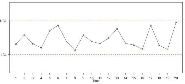
1.1 A sample control chart with upper and lower control limits depicted by the red dashed lines. . . 3
2.1 Two Shewhart control charts (a) and (b) which illustrate the inability of the M: 4/5 scheme to give signals for persistent shifts. . . 15 2.2 A Shewhart control chart of individual data points collected at equally
spaced sampling intervals from time point t = 1, ...,20. This chart is used to illustrate the mechanism of the adaptive r-out-of-m scheme at t= 20. . . 17 2.3 ARL0 values obtained for a process whose IC distribution is N(0, 1),
the threshold valueγ ranges from 0 to 0.1 and ˜α= 0.1 . . . 25
3.1 Distribution of thep-values of aN(0, 1) process where different values of w were used in the computation of ˆσ = d s¯
3(w) during the Phase-I SPC. 44
3.2 AATS values of the control chart (3.15)-(3.16) with the dynamic sam-pling interval (3.5) for monitoring a process whose IC distribution is N(0,1) with mean shift of size {0,0.1,0.5,0.75,1.0,1.5,2,2.5,3} occur-ring at the initial observation time. For the dynamic scheme, two cases are cosidered− (a) λ= 0 and (b) λ= 0.5. In both cases, the value of a is cosidered to be {0,0.2,0.4,0.6,0.8,1.0} and b is chosen to achieve ARL0 = ATS0 = 400. . . 46
pling interval (3.5) for monitoring a process whose IC distribution is N(0,1) with mean shift of size {0,0.1,0.5,0.75,1.0,1.5,2,2.5,3} occur-ring at the initial observation time. For the dynamic scheme, two cases are cosidered−(a) λ∈[0,10] and (b)λ∈[2,10]. In both cases, a= 0 when λ > 0, a = 1 when λ = 0 and b is chosen to achieve ARL0 =
ATS0 = 400. . . 47
3.4 Phase-II monitoring times (in seconds) of the traditional Shewhart chart and the Shewhart chart with a dynamic sampling scheme for an IC process distribution ofN(0, 1) of several sizes n. . . 48 3.5 AATS values of the Shewhart chart with a dynamic scheme and the
Traditional Shewhart chart, where ARL0 = ATS0 = 1,000. In this
example, the parameters of the IC distribution are unknown. In plot (a), the parameters are estimated using the bootstrap approach. In plot (b), we compute the parameters using the distribution estimation approach. . . 52 3.6 Control chart for monitoring the simulated univariate process
observa-tions. The warning lines are the control limits for the chart obtained at a significance level of α= 0.001. . . 54
4.1 Values of σ2
En as given in the expression of (4.2) for n = 1, ...,100, in
cases when σ2 = 1, and ν= 0.02, 0.05, 0.1, or 0.2. . . 63
4.2 p-values of the empirical distribution for the charting statistic (4.4) when n= 10, 20, 30, 50, 100, 200 and 500. . . 64
interval (3.5) for monitoring a process whose IC distribution is N(0,1) with mean shift of size{0,0.05,0.1,0.2,0.4,0.6,0.8,1,1.5,2} occurring at the initial observation time. For the dynamic scheme, two cases are cosidered - (a) λ = 0 and (b) λ = 0.5. In both cases, the value of a is cosidered to be {0,0.2,0.4,0.6,0.8,1.0} and b is chosen to achieve ARL0 = ATS0 = 200 and ν = 0.05. . . 65
4.4 AATS values of the control chart (4.4) with the dynamic sampling interval (3.5) for monitoring a process whose IC distribution is N(0,1) with mean shift of size{0,0.05,0.1,0.2,0.4,0.6,0.8,1,1.5,2} occurring at the initial observation time. For the dynamic scheme, two cases are cosidered − (a) λ ∈ [0,10] and (b) λ ∈ [2,10]. In both cases, a = 0 when λ > 0, a = 1 when λ = 0 and b is chosen to achieve ARL0 =
ATS0 = 200 and ν= 0.05. . . 67
4.5 ARL1values of the EWMA chart when ARL0= 10,000,ν = 0.01, 0.05, 0.2
and the shift size changes from 0 to 3 with a step of 0.1 . . . 68 4.6 AATS1 values of the control chart (4.6)-(4.7). The sampling interval
of S-EWMA is given byd(·) = 1 while the sampling interval for DyS-EWMA, is given by the expression in (4.8). In plot (a), the p-value of the charting statistic is computed using the bootstrap approach. In plot (b), the p-value is computed by the distribution estimation approach. Here,ν = 0.05, and ATS0 = 400 . . . 71
4.7 The DyS-EWMA control chart for monitoring the simulated process data described in Section 4.5. The red warning line represents the significance level,α = 0.00159 which achieves ATS0 = 1,000. . . 73
SPC– Statistical Process Control
IC – In-Control
OC – Out-of-Control
ARL – Average Runlength
ATS – Average time to Signal
AATS – Adjusted Average Time to Signal
CUSUM – Cumulative Sum
EWMA – Exponentially Weighted Moving Average
SS – Standard Shewhart
DyS-S – Dynamic-Sampling Shewhart
DyS-CUSUM – Dynamic-Sampling Cumulative Sum
DyS-EWMA – Dynamic-Sampling Exponentially Weighted Moving Average
CHAPTER 1
BACKGROUND
1.1
Introduction
Recent developments in science and technology have given birth to the big data era in which large volumes of data are consistently being generated from several sequential processes. From health care, manufacturing and production lines, network systems, Internet services, E-commerce and so on, the proliferation of data from these sequential processes has elicited the need to develop innovative methods capable of monitoring these processes. In most cases, the observations from these processes are obtained at individual time points, and they can be described as a random sample from a parametric statistical distribution.
a production line. In this sense, certain quality characteristics of the product from the routine processes are checked to ensure they meet some desired requirements.
Statistical Process Control (SPC) provides statistical tools which are employed to visualize patterns, monitor, and detect shifts (changes in parameters and/or statistical distribution) in a sequential process. The variation in a sequential process can be attributed to two basic sources−common cause variation and the assignable (special) cause variation. Common cause variation results from uncontrollable and unavoidable random variation in a production process which can only be eliminated by changing the entire process, while assignable cause variations are due to malfunction of certain components of the sequential process. When the variation in the production process is due to only common causes, we say that the process is in-control (IC), while if the source of variation in the process results from any assignable cause, we say the process is out-of-control (OC). The main idea behind SPC is to monitor the sequential process and detect when such a system has shifted from being IC to OC.
Figure 1.1: A sample control chart with upper and lower control limits depicted by the red dashed lines.
1.1.1 The Average Run Length
Given the varying underlying assumptions for the implementation of the different control charts to be presented later, the performance of each control chart varies to a significant extent. In order to evaluate the performance of the control charts, the average run length (ARL) has been used extensively in the literature. The run length of a chart can be defined as the number of process readings considered to be IC before an OC reading is observed. Thus, the average run length is the expected number of points plotted on the chart until an OC signal is obtained. An IC ARL, denoted as ARL0, is the ARL associated with a zero-valued shift (an IC data set is being
analyzed). Since there should be no shift when an IC dataset is analyzed, ARL0
represents the number of observations until a false OC signal is given. In contrast, an OC ARL, denoted as ARL1 is the ARL associated with a non-zero shift. It represents
Type-I and Type-II error probabilities in hypothesis testing. In the SPC literature, we usually fix the ARL0 at a given level and try to make the ARL1 value as small as
possible. In other words, we fix the false-alarm rate and then minimize the chance of missing an actual shift.
1.1.2 Phase-I and Phase-II monitoring
Generally speaking, the monitoring of process observations can be categorized into two phases, the Phase I and Phase II monitoring. Each phase has a distinct objective. For the Phase-I SPC, data from a sequential process are collected and analyzed in a backward-looking fashion. This retrospective analysis of the process observations aims at estimating the distribution of the sequential process and also getting the control limits for the control charts to be used in subsequent analysis. This is usually done by understanding the relationship between certain controllable input variables and the quality characteristics of interest. The controllable input variables are then set at optimal values and a set of process observations is collected and analyzed with the trial control limits. If a fault is noticed while monitoring the observations, the OC observations are investigated and discarded. Then, the input variables are re-adjusted and a new set of observations is collected and analyzed. This process of fine-tuning the controllable input variables and constructing control limits is done repeatedly until all assignable causes of variation have been eliminated, thus making the process stable, then clean data are obtained from the process.
subsequent observations obtained from the quality characteristic of interest. However, adaptive charts recalculate the control limits as more observations are collected.
In addition, a distributional shift in the sequential process can either be transient or persistent. If the shift is transient, the process goes OC but thereafter returns to being IC without any intervention. For persistent shifts, when the process leaves the IC state, it remains OC or even goes farther away from the IC state until a corrective intervention is made.
1.2
Traditional SPC charts
The SPC framework has several control charts for detecting several kinds of distributional shifts in a production process. In this section, we give a brief overview of some commonly used charts. The control charts discussed here are primarily used for the Phase-II SPC (in other chapters involving the corresponding charts, the case for the Phase-I SPC is discussed). Also, we assume that the quality characteristic of interest is univariate and numeric observations from this quality characteristic are obtained at equally spaced time points.
Consider the following independent observations obtained from the Phase-II mon-itoring of the sequential process
X1, X2, ...Xτ ∼N(µ0, σ2)
Xτ+1, Xτ+2, ... ∼N(µ1, σ2)
whereτ is an unknown change point,µ0 and µ1 are the respective IC and OC means
of the process (µ0 6=µ1), andσ2 is the process variance. In order to describe the SPC
to be presented can also be modified to give signals for shifts in the variance and shifts in both mean and variances of the process. Also, the IC parameters,µ0 andσ2,
are usually unknown and should be estimated in the Phase-I SPC. With the process defined above, we begin the discussion of the charts.
1.2.1 The Shewhart Control Chart
Developed by Walter A. Shewhart in 1931, the Shewhart chart is a control chart based on the framework of hypothesis testing. The upper, center and lower control limits of the Shewhart control chart are defined as
U =µ0+Z1−α/2 σ; C =µ0; L=µ0−Z1−α/2 σ (1.1)
whereαis the significance level andZ1−α/2 is the (1 - α/2)th quantile of the standard
normal distribution. At time point n, the Shewhart control chart gives a signal for a mean shift if
Xn< L or Xn> U (1.2)
Due to its simplicity, ease of implementation and interpretation of results, the She-whart chart has gained a wide range of applications in industrial processes. The chart has proven to be efficient in detecting large and transient shifts in the mean of the process, this makes it appealing to the Phase-I SPC where such shifts are usually encountered.
the Shewhart chart works under the assumption that the process observations are normally distributed.
1.2.2 The Cumulative Sum Chart
In other to overcome the inability of the Shewhart chart to detect small and per-sistent in a process, Page [20] proposed the CUSUM chart which uses historical data to evaluate the performance of the sequential process at each time point. Historical data may contain vital information about the IC and OC performance of the process. The charting statistic of the CUSUM chart is based on the cumulative sum of the observation at the current time point and previous time points. This is given as
Cn = n
X
i=1
(Xi−µ0) = Cn−1+ (Xn−µ0) for n ≥1, (1.3)
where Cn = 0. In order to detect upward and downward shifts in the process, (1.3)
can be written as
C+
n = max 0, C +
n−1+ (Xn−µ0)−k
Cn− = min 0, Cn−−1+ (Xn−µ0)−k
(1.4)
The CUSUM control chart gives an OC signal for a mean shift in the process if
Cn+ > h or Cn− <−h, forn ≥1, (1.5)
where k > 0 is a pre-specified reference parameter, and h > 0 is a control limit chosen to achieve a desired ARL0 value. The Cn+(Cn−) resets to 0 whenever there is
the process observations are normally distributed. In Chapter 3, we provide more discussion on the performance and implementation of the CUSUM control chart.
1.2.3 The Exponential Weighted Moving Average Chart
Another chart that circumvents the inability of the Shewhart chart to detect small and persistent shifts is the EWMA chart. This control chart which was proposed by Roberts [24] uses historical data to evaluate the performance of the process. The charting statistic of the EWMA chart is based on the weighted average of observation at the current time point and previous observations. This is given as
En =νXn+ (1−ν)En−1 for n≥1, (1.6)
where ν ∈(0, 1] is a pre-specified weighting parameter, and E0 =µ0. And to detect
upward and downward shifts in the mean of the process, we write (1.6) as
E+
n = max 0, ν(Xn−µ0) + (1−ν)En+−1
En− = min 0, ν(Xn−µ0) + (1−ν)En−−1
(1.7)
The chart gives an OC signal for a mean shift if
En+ > ρU
r
ν
2−ν or E −
n < ρL
r
ν
2−ν, for n≥1, (1.8)
where ρL, ρU > 0 is a parameter chosen to achieve a desired ARL0 value. Just like
process observations are not normally distributed.
1.2.4 Other SPC Control Charts
From Section 1.1, we notice that for the SPC problem, the univariate process has a common distribution before a shift occurs (IC distribution) and another distribution (OC distribution) after the shift occurs at an unknown time point. Change point detection (CPD) is a research area in the field of statistics that seeks to detect the specific position at which the distribution of a sequence of random variables changes from one to another. In the literature of CPD, the sample sizes are usually fixed and the distributions follow a parametric nature. Since the number of observations in the Phase-II SPC increases sequentially, change point detection cannot be directly applied to the SPC problem. However, on going research ([9], [10]) in SPC have modified CPD methods to handle the SPC problem and thus, CPD charts have been developed for the detection of distributional shifts in a sequential process.
The measurements from a quality characteristic of interest could be continuous, discrete or categorical. The charts presented in the previous sections focused on the case when continuous numerical observations are available. In cases when the quality characteristic is categorical or discrete but the number of different observations is small, control charts for categorical quality characteristics exist for monitoring the process. Examples of these charts include control charts for monitoring the proportion of non-conforming products of a production process and control charts for monitoring the number of defects in an inspection unit.
of the product. Multivariate version of Shewhart, CUSUM, EWMA and CPD charts exist for detecting shifts in the mean and covariance matrix of the distribution of a multivariate production process.
Furthermore, for cases where the process observations are correlated, the CUSUM and the EWMA chart can be modified to handle such scenarios. Also, for monitoring a process when non-normal data are observed, several non-parametric charts have been developed. These include rank based non-parametric control chart which is based on ranking or ordering of information in the observed and non-parametric control chart by categorical data analysis which is based on observation categorization.
1.3
SPC and Big Data Analysis
A data stream can be simply defined as a constant stream of data flowing from a particular source. This includes data from a sensory machine, data from complex industrial and agricultural machines, data from web services or data from social media websites. In this case, each data is generally timestamped or geo-tagged. Furthermore, we define a stream as a possibly unbounded sequence of data items or records. These data items may be independent of each other or correlated with each other. In this setting, each data item is treated as an individual event in a synchronized sequence [14].
up with the pace at which process readings become available and therefore fail to give a signal for a distributional shift as early as possible. Considering this scenario, it becomes imperative to design and modify traditional control charts so that the complexity of monitoring large volumes of data is minimized and the run time of the monitoring process is reduced.
In order to improve the efficiency of SPC charts for monitoring big data processes, we use some existing methods in the literature to modify SPC charts. Particularly, we use p-values to design control charts and with the information obtained from the p-values, we skip observations that are IC during the monitoring procedure. The dynamic sampling scheme [15] will be used to determine how many observations are to be skipped during the monitoring procedure. Despite the goal of reducing the run time of the charts, we also intend to maintain the ability of the charts in quickly detecting distributional shifts.
1.4
Overview of Thesis
CHAPTER 2
AN ADAPTIVE
R
-OUT-OF-
M
CONTROL CHART FOR
DETECTING SMALL AND PERSISTENT PROCESS
MEAN SHIFTS
2.1
The
r
-out-of-
m
control chart
It well-known that the Shewhart chart does not perform well in detecting small and persistent distributional shifts. This is because it does not utilize historical data which may contain useful IC and OC information during when evaluating the performance of a production process. In order to increase its sensitivity to small shifts, the Shewhart chart is usually implemented alongside with several other supplementary criteria.
Shewhart chart.
To overcome the problem of the increase in the false alarm rate of the sensitivity rules, Klein [13] proposed two alternative schemes based on the standard runs rules. In the first scheme called the two-of-two scheme, the control chart gives an OC signal if two successive points plot above (below) an upper (lower) control limit. In the second scheme, called the two-of-three scheme, the control chart gives an OC signal if two of three successive points plot above (below) an upper (lower) control limit. The control limits for these schemes are symmetric and were estimated in such a way that the schemes have the same IC ARL as that of the standard Shewhart chart. His study shows that both schemes have better ARL1 performance than the Shewhart
chart for process mean shifts up to 2.6σ and they can be easily implemented.
In another study, Khoo [12] noted that obtaining the control limits for the two-of-three scheme proposed by Klein would be difficult for quality control engineers and thus proposed a more user-friendly approach. Khoo expounded on Klein’s approach by using a simulated study to evaluate the performance of various schemes. In this setting, the analyst chooses a pre-specified ARL value for a zero-mean shift, and then obtain the control limits from the simulated values using less tedious steps. Khoo studied the 2-of-2, 2-of-3, 2-of-4, 3-of-3, and 3-of-4, amongst which he concluded that the 3-of-4 had the best ARL performance for small to moderate process mean shifts.
(below) the upper (lower) control limit which are separated by at most (m−r) points placed between the center line and the upper (lower) control limit. They suggested that the M: r/5 scheme were more reliable for detecting small to moderate process mean shifts.
Despite the good performance of these schemes in detecting small mean shifts, they do not perform well in detecting persistent mean shifts because of their inability to use sufficient history data during the monitoring procedure. In the case when the sequential process is IC, and additional less severe and persistent assignable causes, shift the process away from the IC mean in an intermittent but yet consistent manner, the modified schemes are not capable of detecting such irregular shifts. For instance, suppose we begin the Phase-II SPC monitoring with the M: 4/5 scheme, this scheme is primed to detect small shifts of about 0.2σ. So in the sequel considerations presented, we assume that the average shift size is not above 0.2σ. At time point t, the scheme looks back through (t −5) + 1 observations to check for observations that are OC within this window. However, if there are less than 4 OC observations (either in the upper or lower region) within any window, the scheme will fail to give an OC signal.
Consider Figure 2.1(a), at time point t = 5, notice that the chart will not give an OC signal despite the fact that the observations at t = 2,3,4 are all OC. In this case, the process keeps on running and the M: 4/5 scheme fails to give any OC signal despite significant sequence of shifts around time points 2 to 4, 8 to 9, and 14 to 17.
Figure 2.1: Two Shewhart control charts (a) and (b) which illustrate the inability of the M: 4/5 scheme to give signals for persistent shifts.
The illustration presented in Figure 2.1 can be generalized to other M: r/m schemes. It may be argued that a simultaneous combination of several M: r/m schemes can be used to detect such persistent shifts, even though this is plausible, this approach would be hindered by the problem of an increase of false-alarms. Fur-thermore, the M: r/mscheme will require prior knowledge of the shift size before any specific scheme can be employed, this may also hinder its usage since the magnitude of the shift size to be encountered in the process is usually unknown in most cases.
In this Chapter, we propose an adaptive r-out-of-m control chart, in which the values of r and m are chosen adaptively. We show that the chart will detect small to moderate persistent mean shifts and efficiently estimate the shift positions in the sequential process.
2.2
Description of the adaptive
r
-out-of-
m
control chart
Suppose
Xi ∼
N(µ0, σ2) if i≤τ
N(µ1, σ2) if i > τ
whereµ0 6=µ1,τ is an unknown shift position and Xi’s are independent observations.
In order to detect small to moderate persistent shifts in the mean of a production process, we use an adaptive sampling procedure. In this sense, we adaptively select r-out-of-m process observations that plot beyond certain control limits. Here, the maximum value of m is set in advance and then, we use an adaptive procedure to obtain the values of r {r ≤ m} at each time point. The Shewhart control chart consists of three regions− the region above the upper control limit, the region below the lower control limit and the region between the two control limits. In this case, we separately consider points that plot in the region above the upper control limit and the points that plot in the region below the lower control limit. We consider points that plot within the control limits to be IC. At each time point t, when m {m ≤ t} observations have been obtained, let us call the number of points that plot in the region above the upper control limit r1, and the number of points that plot in the
region below the lower control limitr2.
Given a preset maximum value of m, we begin monitoring the process in a retrospective fashion. Thus, at each time point t, for each unit increase from 1 tom, we obtain the values of r1(r2) that plot beyond the upper(lower) control limit.
Also, for each value ofr1(r2) obtained at time point t, we compute the probability of
observing a more extreme value of r1(r2) given that the process is IC. By statistical
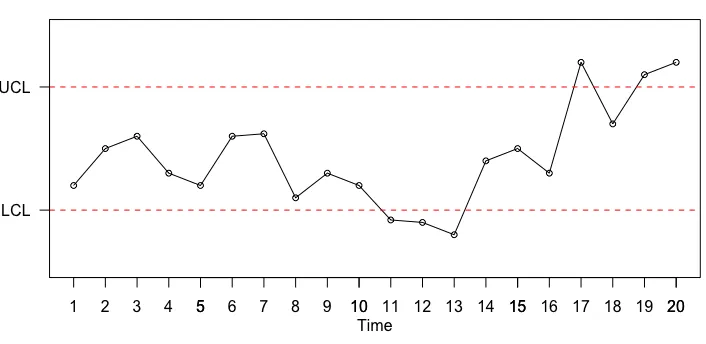
Figure 2.2: A Shewhart control chart of individual data points collected at equally spaced sampling intervals from time pointt= 1, ...,20. This chart is used to illustrate the mechanism of the adaptive r-out-of-m scheme att = 20.
Let us define the random variables X1 and X2 to be the number of points that
plot beyond the upper and lower control limits respectively. Following the assumption that the process observations are independent, it is easy to see that we can model the adaptive r-out-of-m scheme by a binomial probability distribution with parameters mand probability of success ˜α, where ˜αis the probability of observing a point beyond the control limit given that the process is IC.
The adaptive r-out-of-m control chart will give an OC signal at time point t if the minimum of the set of p-values for different m obtained for r1(r2) is less than a
threshold valueγ. This threshold value γ is obtained in such a way where a pre-fixed ARL0 value is achieved. For instance, consider the process which is visualized in
of m, the minimum p-values associated with the respective random variablesX1 and
X2, indicate an extreme case.
From Table 2.1, when m = 4, r1 = 3. The p-value at such instance is computed
as
P1 =P(X1 ≥r1) = 1−P(X1 ≤(r1−1)) = 1− r1−1 X k=0 m k ˜
αk(1−α)˜ (m−k)
P(X1 ≥3) = 1−
(
4 0
(0.1)0(1−0.1)(4−0)+
4 1
(0.1)1(1−0.1)(4−1)
+
4 2
(0.1)2(1−0.1)(4−2)
)
= 1− {0.6561 + 0.2916 + 0.0486}= 0.004
From Table 2.1, it is easy to see that 3-out-of-4 and 3-out-of-10 OC observations correspond to the minimum p-values in the upper and lower regions respectively. Thus, the control chart will give an OC signal at this time point if either of the minimum p-value is less that the pre-fixed threshold value γ.
Table 2.1: r1, r2, and m alongside their corresponding p-values for the process
depicted in Figure 2.2. This illustrates the mechanism of the adaptive r-out-of-m chart at time, t= 20.
m r1 P(X1 ≥r1) r2 P(X2 ≥r2)
1 1 0.100 0 1.000
2 2 0.010 0 1.000
3 2 0.028 0 1.000
4 3 0.004 0 1.000
5 3 0.009 0 1.000
6 3 0.016 0 1.000
7 3 0.026 0 1.000
8 3 0.038 1 0.570
9 3 0.053 2 0.225
10 3 0.070 3 0.070
In the subsequent sections, we provide pseudo codes when using the adaptive r-out-of-m control chart, particularly for detecting OC signals, estimating the ARL0
values and obtaining the threshold value γ for some certain ARL0 values.
2.2.1 Pseudo Code for detecting an OC signal
Let ˜αbe the pre-specified probability of observing a point beyond the control limit given that the process is IC. Also, letγ be the pre-specified threshold value which is chosen to achieve a given ARL0 value. Let n be the number of observations in the
sample and m the number of most recent observations we wish to consider. In the i-th iteration, for m ≤i≤n,
Step (1) • In thej-th iteration, for 1≤j ≤m, obtain the number of points, r1j,
that plot above the upper control limit, and the number of points, r2j, that plot below the lower control limit.
P1j =P(X1 ≥r1j) = 1−P(X1 ≤(r1j−1))
= 1−
r1j−1
X l=0 j l ˜
αl(1−α)˜ (j−l)
P2j =P(X2 ≥r2j) = 1−P(X2 ≤(r2j−1))
= 1−
r2j−1
X l=0 j l ˜
αl(1−α)˜ (j−l)
Step (2) If min(P1j, j = 1,2, ..., m) < γ or min(P2j, j = 1,2, ..., m) < γ, print out
the values ofitogether with the corresponding values ofrandm, andstop
the algorithm. Otherwise, i=i+ 1, and return to step (1).
For the adaptive scheme, the control limits will be determined by the value of ˜α. For instance, ˜α = 0.0027 yields 3-sigma control limits. In the case of the standard Shewhart chart, the value of ˜α determines the ARL0 value, where ARL0 = α1˜. Here,
the run length of the process follows a geometric distribution with parameter, ˜α. However, since the proposed adaptive scheme follows some other criteria for giving an OC signal, the ARL0 is computed differently. In the literature, the Markov chain
approach has been extensively used to obtain the ARL0 values for several runs rules.
However, considering the fact the scheme proposed in this study follows an adaptive nature and the value of m may vary (it could be large), we resort to simulation for estimating the ARL0 value. Certainly, computational complexities will arise if
we compute the ARL0 value using the conventional Markov chain approach. This
is because there will be too many transient states in the Markov chain, thus the transient space may be totally large and out of computation ability.
In this study, Monte Carlo simulations are used to estimate the ARL0 value. We
to understand several properties of the ARL. The algorithms given in Sections 2.2.2 and 2.2.3 closely follow the methods described by ([21], page 127 and 129). Sec-tion 2.2.2 provides a stepwise process to compute the ARL0 value.
2.2.2 Pseudo Code to Compute an Estimate of the ARL0 Value
Let R be the number of replicated simulations. In order to obtain stable values, this number should be a large positive integer. Specify the values of ˜α and γ. In the g-th replicated simulation for 1≤g ≤R,
Step (1) Generate n observations from N(0, 1)
Step (2) Compute the run length RL(g) by the following loop; for m≤i≤n
• Compute the necessary values from Section 2.2.1.
• From step (ii) in Section 2.2.1, if min(P1j, j = 1,2, ..., m) < γ or
min(P2j, j = 1,2, ..., m) < γ, which indicates an OC signal, set
RL(g) = i and break out of the loop; otherwise, let i = i+ 1 and continue the loop.
Step (3) Proceed tog =g+ 1, and return to step (1) until R is reached.
Step (4) The ARL0 is the average of R run length values. i.e ARL0 =
PR g=1RL(g)
R .
In subsequent sections, we provide some interesting properties of the ARL0.
Nonethe-less, we see that the ARL0 value depends on the threshold value γ. Thus, it becomes
imperative to obtain the threshold value which will yield a certain ARL0 value. We
utilize the bisection method to search for the threshold value which reaches the expected ARL0 to a certain accuracy. The algorithm presented in Section 2.2.3 below
2.2.3 Pseudo Code to Search for the Threshold Value
Let A0 be the pre-specified ARL0 value and let [γL, γU] be the interval from
which the threshold value, γ is searched. Let ρ > 0 be a small number denoting the estimation accuracy of the search. Set R to be the number of replications used in obtaining the run length of the process. SetM to be the number of required iterations for the search, and then for 1≤j ≤M perform the following steps iteratively.
Step (1) Compute γ = (γL+γU)/2. Using γ
• For 1 ≤g ≤R, compute the run length, RL(g). • Set ARL0 = mean(RL)
Step (2) If the ARL0value obtained from step (1) lies in the interval [A0−ρ, A0+ρ],
stop the algorithm. Thus, the value of γ obtained from step (1) is the searched value. Otherwise, set
γL =γL; γU = (γL+γU)/2 for ARL0 > A0
γL = (γL+γU)/2; γU =γU for ARL0 < A0
continue toj + 1, and return to step (1).
If the algorithm does not stop before or atM-th iteration, then the value of the ARL0
obtained still lies outside the interval [A0−ρ, A0+ρ]. Thus, the estimation accuracy
specified by ρ cannot be reached.
In order to choose optimal starting values (γLandγU) for the search, we make sure
that the pre-specified value,A0, lies well in the interval of ARL0 values obtained when
The magnitude of the estimation accuracyρshould be small, a number in the interval [0, 1] is usually chosen.
2.3
Performance of the
r
-out-of-
m
scheme
Large values of ˜α and γ will detect small and transient shifts in the process. In this setting, the control limits will be constricted and the scheme frequently yields small combinations of r-out-of-m observations that plot beyond the control limits such as 1-out-of-2, 2-out-of-2, 2-out-of-4, and 2-out-of-5. Since the resulting p-values will be small and may be often less than the threshold value, the ARL performance of the process will be poor, and thus there will be substantial false alarms. However, the adaptive scheme is advantageous in the sense that we can reduce the threshold value in order to detect persistent shifts and also reach some larger ARL values. In a similar fashion, small values of ˜α are primed to detect large and transient shifts. Also, the value of the threshold can be set to achieve certain ARL values and detect long-staying shifts in the process.
Furthermore, from numerical experimentation shown in Table 2.2, we observe that the maximum value of m chosen for the r-out-of-m scheme does not have a substantial impact on the ARL performance. Given the values of ˜α and γ, we see that the variation in the ARL0 values for increasing values ofm is very minimal.
Table 2.2: ARL0 values obtained for several maximum values of m used in the
adaptive r-out-of-m scheme. In this case ˜α= 0.1 andγ = 0.01.
m 5 7 10 12 15 20 25 30
ARL0 800.9 798.6 738.2 741.0 739.6 742.0 732.0 743.3
5 because such shifts will only require information around the current time point. While for persistent shifts, m should be set to at least 10, because such shifts will require sufficient history data.
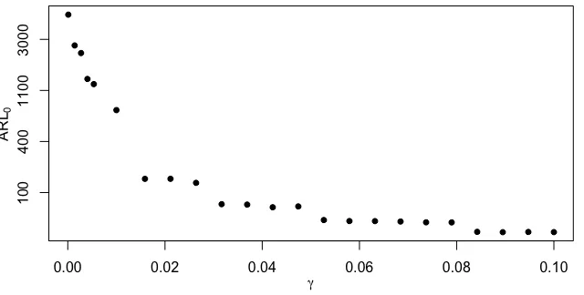
Next, we investigate the ARL performance of a process whose distribution is N(0, 1). In this setting, we select ˜α = 0 and γ is chosen from the interval [0, 0.1]. The obtained ARL0 values are displayed in Figure 2.3. From this process, we observe
that as γ increases, the ARL0 value decreases. Furthermore, notice the jumps in the
ARL0 values displayed in Figure 2.3, the gaps grow farther apart when theγ is small.
In this setting, we discovered that certain ARL0 values will not be achieved when
the adaptive scheme is employed. This is one limitation of the adaptive r-out-of-m scheme, in subsequent sections, we provide a detailed discussion of this limitation and a potential approach to overcome it.
In addition, we present the threshold values obtained for some commonly used ARL0 values in Table 2.3. For this illustration, the maximum value of m is set to be
10, and we assume that the process is N(0, 1). Notice that for some slight change in γ, especially when this value is small, there seems to be significant jumps in the resulting ARL0 values.
2.4
Limitations of the Adaptive
r
-out-of-
m
Scheme
From the description of the adaptive r-out-of-m chart provided earlier, we indi-cated that at each time point t, the minimum of a set of p-values is compared to a pre-fixed threshold value γ. That is, if min(Pt1j, j = 1, .., m) or min(Pt2j, j =
Figure 2.3: ARL0 values obtained for a process whose IC distribution is N(0, 1),
the threshold value γ ranges from 0 to 0.1 and ˜α = 0.1
pointt, we obtained 3-out-of-5, and 3-out-of-6 whenm= 5 and 6 respectively. There will be a jump in the resulting p-values for both cases because of the discrete nature of r and m. So, when the maximum value of m is fixed, we can only attain certain p-values for different combinations ofrand m. Since we are checking if the minimum of thesep-values is less than γ, there will be substantial impact of the discreteness of the charting statistic on the performance of the chart, i.e. the ARL0. This limitation
is presented in the graph displayed in Figure 2.3. This explains why we may not be able to obtain specific ARL0.
Since specific ARL0 values may be desired by practitioners using SPC charts, this
limitation may pose a challenge to its usability and acceptance. If the threshold value required to reach some specific ARL0 values cannot be computed, such monitoring
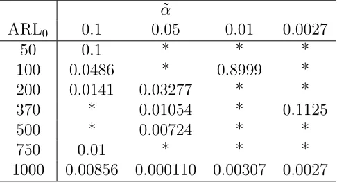
Table 2.3: Computed threshold values, γ of the adaptive r-out-of-m scheme de-scribed in Section 2.2 for some commonly used ARL0 and ˜α values. * denotes thatγ
could not be obtained for such combination of ARL0 and ˜α
˜ α
ARL0 0.1 0.05 0.01 0.0027
50 0.1 * * *
100 0.0486 * 0.8999 *
200 0.0141 0.03277 * *
370 * 0.01054 * 0.1125
500 * 0.00724 * *
750 0.01 * * *
1000 0.00856 0.000110 0.00307 0.0027
CHAPTER 3
DYNAMIC SAMPLING SCHEMES
3.1
Introduction
In Section 1.2, we introduced some commonly used SPC charts. The traditional versions of these charts are designed to monitor each and every observation during the monitoring procedure.
provide information about the potential of a distributional shift in the process. In this sense, the information obtained from the p-value at each time point can be used to adjust the sampling scheme of the monitoring process. That is, the sampling time and the sampling size of the next sample will be dependent on the magnitude of the p-value of the charting statistic at the current time point. This approach enables the practitioner to make informed decisions when handling future observations. For instance, if the p-value is much larger than α, this provides sufficient evidence that the process is likely to be stable at such time point.
In this context, since subsequent sampling decisions will be dependent on this numerical measure, variable sampling rates (VSR) rather than conventional fixed sampling rates (FSR) − which depends on fixed time intervals or sample sizes − will be incorporated in the design of traditional SPC charts. The VSR is somewhat analogous to the adaptive SPC control chart, a control chart in which either the sampling interval or the sampling size (or both) can change depending on the value of the charting statistics [18]. As discussed in the literature, one notable advantage of the VSR over the FSR is that, given the IC ARL0 and the IC average sampling
rate, the VSR has good performance in detecting small to moderate shifts.
The VSR scheme depends on several features which are changed according to state of the process at the current time point. A typical VSR scheme would depend on either the variable sampling interval (VSI), the variable sampling size (VSS) or both variable sampling interval and variable sampling size (VSSI).
plots beyond the control limits. On the contrary, if the sample point plots within the central region, the control chart with the VSI delays the next batch, and for the VSS chart, fewer observations are taken in the next batch. In this case, the VSSI combines both methods again [7].
While taking into account the potential shift size in a process, several researchers have suggested a variety of methods to adaptively control subsequent sampling times during the Phase-II SPC. The VSI schemes were introduced by Reynolds et al. [23], and were also implemented in the ¯X chart. Reynolds et al. [22] also proposed VSI schemes for CUSUM charts. In this case, the sampling interval, d(·), is defined to equal either one of two values (d1 or d2) based on the membership of its charting
statistic in a specific region defined by its control limits. More recently Li and Qiu [15] proposed the dynamic sampling interval scheme which is defined as a continuous function of the p-value of a charting statistic. These sampling interval schemes form the framework of some VSI control charts used for the detection of potential but unknown mean shifts in the distribution of a production process. The VSI schemes allow the sampling time to be changed according to the current state of the process readings.
DyS-CUSUM chart uses thep-value of the CUSUM chart in its design. However, both VSI-ACUSUM and DyS-CUSUM charts use the adaptive selection of the reference value of the CUSUM chart which was developed by [26].
Numerical studies shown in [15] shows that in general, the DyS-CUSUM chart has the advantage of quickly detecting certain shift sizes when compared to the VSI-ACUSUM chart. This means that the dynamic sampling scheme has better performance than the conventional 2-interval sampling scheme. Thus, our study focuses on the incorporation of the dynamic sampling schemes in other conventional SPC charts. We emphasize this method because of its computational efficiency and optimal performance when handling different shift sizes.
Among popular SPC charts with a fixed ARL0 value, the CUSUM chart has
optimal performance − the lowest ARL1 − for detection of distributional shifts
in a production process that is normally distributed if the reference value k of its charting statistic is chosen properly for a particular shift size [19]. Nevertheless, if the production process follows some other distribution that is not normal, the CUSUM chart does not perform well in detecting distributional shifts. Specifically, the CUSUM chart is sensitive to the assumption that both the IC and OC distributions of the sequential process are normally distributed [6]. In most real-world applications, the distribution of the production process is usually unknown, hence it becomes imperative to derive dynamic sampling schemes for other control charts which are robust to the normality assumption.
3.2
The Dynamic Sampling Scheme for the CUSUM chart
We begin the discussion with the design of the CUSUM control chart using p-values. For this design, let us assume that the IC process distribution is known. Li et al. [16] provide a rigorous discussion of this design which is presented below. The p-value of the charting statistic of the CUSUM chart is described as follows.
Suppose we have a sequence of independent Xi observations from a production
process, where
X1, X2, ..., Xτ ∼N(µ0, σ2), if the process is IC
Xτ+1, Xτ+2, ...∼N(µ1, σ2), if the process is OC
where τ is an unknown change point in the mean of the process, and µ0 6= µ1, and
σ02 = σ12 = σ2. Then as shown in (1.4), the charting statistic of the conventional CUSUM chart for detecting an upward mean shift is defined by
C0+ = 0
C+
n = max(0, C +
n−1+ (Xn−µ0)−k)
(3.1)
If reference parameterk is chosen as (µ1−µ0)/2 = δ/2, then the chart is optimal for
detecting the particular shift µ1. The chart gives a signal of an upward mean shift
when
Cn+> h (3.2)
the charting statistic of the CUSUM chart is described as follows. Let C+∗
n be the
observed value of the charting statistic Cn+, then the p-value at the n-th time point is defined by
PC+∗
n =P(C + n > C
+∗
n ) (3.3)
We would conclude that the process has gone out-of-control at the n-th time point if
PC+∗
n < α (3.4)
α? The waiting time to observe the next sample is dependent on the sampling interval functiond(·). Logically, thed(·) should be an increasing function of thep-value, that is, d(·) increases as PC+∗
n increases. We proceed by describing the sampling interval
function proposed by Li and Qiu [15]. Their sampling interval function is chosen from the Box-Cox transformation family and is defined as
d(PC+∗
n ) =
a+bPλ
C+n∗ if λ >0
a+blog(PC+∗
n ) if λ= 0,
(3.5)
3.2.1 Estimation of Parameters
In order to estimate the parameters a, b, and λ in the sampling interval d(·), Li and Qiu [15] carried out several simulation studies to obtain optimal values for these parameters. The authors primarily used the AATS1 as a measure of the performance
of the control chart for detecting several shift sizes. In this section, we provide a brief overview of the results provided by the authors.
For their numeric experimentation of the parameter a, the authors chose a to be in interval [0, 1], negative values ofa, could result to negative values for the sampling interval. Also, when λ > 1, d(PC+∗
n ) would be consistently larger than 1 if a > 1.
This would not be ideal when a potential shift has been observed. When λ = 0, a was chosen to be 1, and when λ > 0, a was chosen to be 0. Using the information from the selection of a, it was shown that the performance of the scheme is almost identical whenλ ≥2. Thus, the authors choseλ= 2. With these chosen parameters, the sampling interval, d(PC+∗
n ), now becomes
d(PC+∗
n ) =b·P 2
Cn+∗ (3.6)
The parameter, b, which can be determined to satisfy the requirement that ATS0
= ARL0, is selected as an integer multiple of the smallest time unit in a specific
application, and thus, the sampling interval needs to be rounded when necessary.
ˆ
δn= max
n
δmin,(1−r)ˆδn−1+r(Xn−µ0)
o
(3.7)
where δmin > 0 is the minimum shift size of interest, ˆδ0 = δmin and 0 < r < 1 is a
weighting parameter. Define kn = ˆδn/2, and the resulting charting statistic becomes
C0+ = 0,
Cn+ = max(0, Cn+−1+ (Xn−µ0−kn)/hn),
(3.8)
wherehn>0 is a control limit. In order to approximately reach a pre-specified ARL0
value, Shu and Jiang [25] provided the following formula to compute the control limit
hn=
log(1 + 2kn2 ·ARL0 + 2.332kn)
2kn
−1.166 (3.9)
These authors provide some practical guidelines for choosing the parametersδmin and
r, and also showed that the CUSUM chart with adaptive selection scheme shown above performs well in various cases.
3.2.2 Calculating the p-values
In order to compute the p-value, PC+∗
n , it is imperative to specify the distribution
of the CUSUM charting statistic,Cn+. Here, two common cases are usually considered − when the IC process distribution is either known or unknown. For the case when the IC process distribution is known, Monte Carlo simulations have been used in the literature to estimate the IC distribution of C+
n. In this setting, random observations
When the IC process distribution is unknown, availability of an IC dataset would be handy in estimating the distribution ofCn+. In this setting, the bootstrap approach is another alternative for estimating the IC distribution ofCn+. Thus, resampled data are repeatedly drawn from the available IC process data, and these resampled data are then used to compute C+
n. This process is repeated as much as B times, after
which theB number of C+
n are used to compute the p-values of the observed charting
statistic,PC+∗
n , in the Phase-II SPC.
Using Monte Carlo simulations, Li and Qiu [15] further showed that their control chart with the adaptively selected reference value kn has the steady-state property
for n ≥ 50. By steady-state, we mean that as the shift time τ increases, the value of AATS1 remains quite stable. In general, the control chart given in (3.8) with the
sampling interval (3.6) is called the dynamic sampling CUSUM chart (DyS-CUSUM).
As stated earlier, we adopt the dynamic sampling approach for monitoring big data processes because it shows to have the best performance in the class of VSI schemes. From this point, we begin the design of other traditional SPC charts using dynamic sampling schemes.
3.3
The Dynamic Sampling Scheme for the Shewhart
Con-trol Chart
3.3.1 The Phase-I SPC
In this Phase, we present an overview of the design of the control limits. Suppose we are have an independent sequence of Xi {i= 1, ..., n} observations with unknown
change point τ. Letµ0 denote the IC mean and σ denote the IC standard deviation
of the process. In this case, we assume that a shift is observed only in the mean of the process, whereas the variance remains stable. Typically, the Shewhart control chart is commonly used when batch data are observed. Nevertheless, under mild adjustments of the charting statistic, the chart can be used to monitor individual observations. In order to employ the control limits of the traditional Shewhart chart to monitor individual observations, we bin the observations into groups using a moving window technique with window size w and a total of n−w−1 groups. Thus, we have
Group 1: X1, ..., Xw
Group 2: X2, ..., Xw+1
.. .
Group n−w−1: Xn−w+1, ..., Xn
Several researchers [21] advise against grouping the observed data in such a way where the first group consists of the first ˜w observations, the second group consists of the next ˜wobservations, and so on; where ˜w >1 is the group size. In this context, it will be difficult for the practitioner to pinpoint the exact time at which the process went OC. Another limitation of this approach is that, the exact ARL0 value which is used
Evaluating the performance of the process at each time point can be constructed as a test of hypothesis problem. That is, we test the following hypothesis
H0 : µ=µ0; H1 : µ6=µ0
where µ denotes the true process mean. Thus, an appropriate test statistics for this hypothesis is given as
Z = Xi−µ0
σ ∼N(0, 1) (3.10)
Given the observed value of the test statistic |Z∗|, the null hypothesis is rejected at a pre-specified level of significanceα if
|Z∗|> Z1−α/2
whereZα/2 is theα/2 critical value of the standard normal distribution. Thus, in this
setting, given the observed data at time point i, the process is said to OC if
Xi < µ0−Z1−α/2 σ or Xi > µ0 +Z1−α/2 σ (3.11)
In practice, the IC mean µ0 and standard deviation σ are usually unknown. Given
the observed values from the process, we estimate the IC mean as
ˆ
µ0 = ¯X =
1 n
n
X
i=1
Xi (3.12)
to Kenney and Keeping [11], this bias depends on w, and thus we have
E
1 d3(w)
si
=σ (3.13)
where si is the sample standard deviation of each moving window with size w, and
d3(w) is a constant that corrects for the bias, and its expression is given as
d3(w) =
2(v−1)(2v−2(v−2)!)2
(2v−3)!
q
2
π(2v−1) if w= 2v (2v−1)!
2(2v−1(v−1)!)2 pπ
v if w= 2v+ 1
notice that 3 ≤ w < 170, otherwise, d3(w) does not exist. Therefore, we have that
the estimate of σ is
ˆ
σ= s¯ d3(w)
where ¯s= n−w+11 Pn−w+1
i=1 si. Some researchers have also used the range of each batch
to estimate σ, however we prefer the sample standard deviation, because for large batch sizes, the range loses statistical efficiency when it is used to estimate σ [18]. Since we have adequate computational resources and w will be mostly large, it is natural to use to the sample standard deviation. Thus, given the estimated parame-ters and by rewriting (3.11) the Shewhart control chart for individual observations is given as
U = ¯X+Z1−α/2 σ;ˆ C = ¯X; L= ¯X−Z1−α/2 σˆ
Xi < L or Xi > U (3.14)
With this modification, the process observations are usually assumed to follow a normal distribution. Borror, Montgomery, and Runger [3] studied the performance of the Shewhart control chart for individual observations when the process observations are not normally distributed. Their study showed that if the process follows some other distribution, then the control limits presented in (3.14) could be inappropriate. Specifically, suppose the IC process follows a non-normal distribution such as the t distribution, Exponential distribution or any other distribution with a long right tail, we notice that the ARL performance for these processes are poor. Forα = 0.0027, the control charts for these distributions yield ARL values that are constantly less than 370 which is the standard ARL value to achieve when this control chart is employed. Therefore, it will be necessary to check the normality assumption before the Shewhart chart for monitoring individual observations can be employed.
3.3.2 Phase-II SPC
In this Phase, we begin monitoring the process observations. After obtaining the control limits and IC dataset from the Phase-I SPC, suppose we have an incoming sequence of independent process observationsYi {i= 1,2,3, ...}with unknown change
pointτ. Again, we assume that random shifts occur only in the mean of the process, whereas the variance remains stable. Now, we begin the monitoring of the sequential process.
with dynamic sampling scheme, we are majorly concerned with the detection of the likelihood of possible mean shifts in the sequential process. The current set up cannot give us vital information about potential mean shifts. In order to make our control chart robust to potential shifts in the process, we proceed by using the p-value of the individual process observation to detect shifts in the mean of the process. Given that the process is IC, the p-value is a measure of the extremity of each sample observation [2]. Thus, it gives us vital information for assessing evidence of a mean shift in the process. For thep-value approach, rather than comparing the observation at each time point with the control limits, we compute the p-value corresponding to each observation and then, compare the obtained p-value at each time point with a pre-specified level of significance α. This comparison replaces the initial decision expression in (3.14) which is used to decide if the process is IC at each time point. The p-value of the observed value Y∗ at the n-th point is defined as
PY∗
n =P
|Z|>
Yn−µ
σ ≈P |Z|>
Yn−X¯
¯ s/d3( ˜w)
(3.15)
where µ and σ are the unknown parameters of the IC distribution. From (3.12), µ0 =E( ¯X), and from (3.13), σ=E
¯ s d3( ˜w)
which are estimated in the Phase-I SPC. The chart gives evidence of an OC mean shift if
PY∗
n < α (3.16)
Indeed, using the p-value approach has several advantages. The most paramount advantage being that it is able to inform the practitioner about the likelihood of a potential shift in the mean of the process. In this sense, if the p-value is way larger than α, which indicates that the process is likely to be stable and likely to remain stable in the near future, the practitioner can delay the time before the next sample is collected or collect fewer observations at the next regular sampling time. In contrast, if the p-value is less than α, this indicates that the process is unstable at such time and the process should be stopped. However, if the p-value is only marginally less than α, this indicates that the process is on its way to be unstable and the chart is likely to give a signal in the near future. In this case, the process may still be allowed to continue running, monitoring of the next sample should be sooner than usual and with the collection of more observations at this sampling time. In each setting presented above, the sampling time is variable and also, it is a function of the p-value. In subsequent sections, we will discuss how the sampling time will be determined.
This approach of skipping observations that are judged to be IC during the monitoring procedure will be highly instrumental for sequential processes generating large volumes of data. Rather than monitoring the observation at each time point, we reduce the complexity of the monitoring procedure by placing more emphasis on time points where potential shifts are noticed. Thus, we are able to reduce the run time of the monitoring procedure while still maintaining quick detection of distributional shifts in the process.
where a pre-specified level of significance is used to judge if the hypothesis should be either rejected or not rejected. Using the decision criteria of (3.16), at each time point, the practitioner will be able to clearly report the status of the process. Also, this approach allows the practitioner to make more informed decisions and take insightful actions in cases when the process is still IC or when a shift has been detected.
In order to compute the p-value at each time point, first, we need to indicate the parameters of the IC process distribution. Given that the IC process distribution family is known, we can estimate the mean and the standard deviation of the IC process distribution from IC observations obtained from this distribution family using the estimation approach described in Section 3.3.1, in whichµis estimated by ¯X and σ is estimated by d(w)¯s . As an alternative to the estimation approach described in Section 3.3.1, we can estimate the parameters of the IC process distribution using the bootstrap approach when IC process observations are available. In this sense, resampled data are obtained by repeatedly drawing observations of size ˜w with replacement from the IC data set. This process is carried out B times, then, the B number of samples are used to estimate the parameters of the IC process distribution. In the same vein, the resampled data can also be used to design the control limits of the Shewhart chart. For approximately large B, and w > 1, the bootstrap method gives a good approximation of the parameters of the IC process distribution.
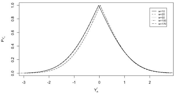
Figure 3.1: Distribution of the p-values of aN(0, 1) process where different values of w were used in the computation of ˆσ= d ¯s
3(w) during the Phase-I SPC.
mean (in this caseµ= 0) in either direction, the correspondingp-value decreases, but the observations clustered about the IC mean have the largest p-values. Therefore using the expression in (3.16), the control chart is more likely to give a signal for a mean shift when observations drift away from their IC mean. Also, since the dynamic sampling scheme is an increasing function of thep-value, we would delay the sampling time of the next observation when we notice that a sequence of process readings are consistently clustered around the IC mean, that is, these sequence of observations have large p-values. However, if the p-value begins to get closer to the significant level, the practitioner is alerted to be become more cautious of the process.
3.3.3 Estimation of the Sampling interval
expression given in (3.5) which is restated below shows the sampling interval function with parameters a, b and λ.
d(PC+∗
n ) =
a+bPCλ+∗
n if λ >0
a+blog(PC+∗
n ) if λ= 0,
Section 3.2 also briefly describes the estimation of these parameters for the CUSUM control chart. Subsequently, we discuss the estimation of the parameters of the dynamic sampling scheme for the Shewhart control chart.
The parameters, a,b andλ will be evaluated using the ATS and the AATS of the Shewhart control chart. For a pre-specified ATS0 value and for a specific shift size,
the optimal chart will be the chart with the least AATS1 value. By convention, we
want to achieve the situation where ATS0 = ARL0. This allows us to estimate the a
and λ and then set b to reach this requirement.
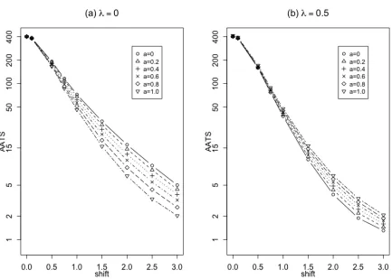
First, we begin by estimating the parameter a. As advised by Li and Qiu [15], let a be chosen from the interval [0, 1]. Let us consider the case when the IC process distribution is N(0,1) with a mean shift at the initial time point of size {0,0.1,0.5,0.75,1.0,1.5,2,2.5,3}. For investigative purpose, let us also consider the cases when λ = 0 and λ = 0.5. Figure 3.2 shows the AATS values of the chart (3.15)-(3.16) when this process is monitored. For the case when λ = 0, the values of AATS1 decrease as the values of a increase, and the chart has the best performance
when a = 1. However, when λ = 0.5, the AATS1 decreases when a decreases, and
the chart performs best when a= 0. Therefore, we set a= 1, when λ = 0 anda = 0 when λ >0.
Figure 3.2: AATS values of the control chart (3.15)-(3.16) with the dynamic sampling interval (3.5) for monitoring a process whose IC distribution is N(0,1) with mean shift of size{0,0.1,0.5,0.75,1.0,1.5,2,2.5,3}occurring at the initial observation time. For the dynamic scheme, two cases are cosidered − (a) λ= 0 and (b) λ= 0.5. In both cases, the value ofais cosidered to be{0,0.2,0.4,0.6,0.8,1.0}and bis chosen to achieve ARL0 = ATS0 = 400.
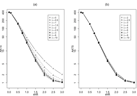
Figure 3.3: AATS values of the control chart (3.15)-(3.16) with the dynamic sampling interval (3.5) for monitoring a process whose IC distribution is N(0,1) with mean shift of size{0,0.1,0.5,0.75,1.0,1.5,2,2.5,3}occurring at the initial observation time. For the dynamic scheme, two cases are cosidered − (a) λ ∈ [0,10] and (b) λ ∈ [2,10]. In both cases, a = 0 when λ > 0, a = 1 when λ = 0 and b is chosen to achieve ARL0 = ATS0 = 400.
The estimated parameters obtained from o