358 | P a g e
EVALUATION AND OPTIMISATION OF OPERATIONAL
CONDITION THROUGH ACO SEED SCATTER SEARCH
ALGORITHM FOR TURNING PROCESS ON AISI 316 L
MATERIALS
Dr.D.Ramalingam
1, Dr.M.Saravanan
2, R.Rinu Kaarthikeyen
3M.Angel Shalini
41
Associate Professor, Nehru Institute of Technology, Coimbatore, (India)
2
Principal, SSM Institute of Engineering and Technology, Dindigul, (India)
3
Research Associate, Manager – Engineering, TCMPFL, Chennai, (India)
4
Research Scholar, Sri Ramakrishna College for Women, Coimbatore, (India)
ABSTRACT
Machining the materials and getting the required range of surface finish within the permissible range is one of the
major setbacks in the manufacturing industries concern. Though there are many conventional metal cutting processes
are there in practices, turning process is the most advantageous machining process and very commonly used by the
manufacturing industries that too with automation and rigidity of the machine tool with high range of speed, feed
improvement. Even then, the factors influencing this surface quality which are many in numbers, the main cutting
condition variables like spindle speed, tool feed rate on the work material, depth of cut given on the material per travel
are the major concerns. Henceforth right selection of such parameters and their suitable combinations are one of the
top priority responsibilities by the operation engineers which are highly possible either through conventional or
evolutionary optimisation techniques. Investigating and optimizing the combination of the input machining parameters
to achieve the desired surface finish is considered as the objective of this presentation with the Ant Colony Optimisation
seed Scatter Search algorithm technique in MATLAB programming. With the Reference to the convergence
performance of the algorithms the hybridization of regression equations feed as input to the programming further
simulation carried out. The outcomes of the results are found to be improved by each phase of the simulation. The
optimum parameter combinations for improved surface finish are identified.
Keywords-
AISI 316L steel material, Turning, Regression, Ant Colony Algorithm, Genetic Algorithm, Scatter
Search Algorithm, Particle Swarm Optimisation, Hybridization, Minitab, MATLAB.
I. INTRODUCTION
359 | P a g e
special applications, the surface finish quality calls to high degree of importance. Any material would have to undergo the machining processes before it attains its final shape and dimension. While such metal cutting operations are being carried out to the final stage, manufacturing to the required surface quality is the quite common issues, because of the variables involving in the machining are having its own impact on the outcome of the processing either individual or in combination. The important input cutting parameters among all are cutting speed, tool feed and the depth of cut in every pass. Henceforth right selection of such parameters and their suitable combinations are one of the top priority responsibilities by the operation engineers, to obtain desired surface quality and also to avoid rejection rate and rework. This investigation primarily aimed onto the analysis and optimisation of cutting variables like cutting speed, feed and depth of cut on the resultant parameter surface roughness.Abbreviations Used
CS Cutting speed GA Genetic Algorithm
DOC Depth of cut R-sq R - square statistical value
Exp Experiment R-sq (adj) R - square adjusted statistical value
f Feed rate R-sq (pred) R - square predicted statistical value
PSO Particle Swarm Optimization Reg Regression
ACO Ant Colony Optimisation Algorithm Ra Surface Roughness
SSA Scatter Search Algorithm
II. LITERATURE REVIEW
360 | P a g e
developed model using genetic algorithm, in order to attain the required surface quality. Tzeng and Chen [9] used grey relational analysis to optimize the process parameters in turning of tool steels. The optimum turning parameters were determined based on grey relational grade, which maximizes the accuracy and minimizes the surface roughness and dimensional precision. The main aim of this investigation is to study the influence of the input machining parameters during turning operation on the average surface roughness of the machined surface. The examination and forecasting of optimized parametric combination is recognized through the application of ACO, PSO, GA and SSA algorithms through MATLAB programming. Also with a new approach as feeding the regression equation relationship as input fitness instead of random selection while simulation.III. EXPERIMENTAL DATA
The properties of the work material AISI 316L steel taken for the experiment is material listed in the Table 3.1. In CNC lathe OKUMA Lb 10II model, a coated tool -DNMG 110402-M3 with TP 2000 coated grade which has rhombic shape with cutting edge angle 55° is used as the cutting tool to conduct the experiment by Nokolaos [12]. The coating on the tool is of four layers of Ti [C, N] + Al2O3 + Ti [C, N] + TiN with the cutting edge angle as 93°.
Table 3.1 Mechanical properties of AISI 316L material
Property Quantity
Hardness, Rockwell B 79 HRB Tensile strength, ultimate 560 MPa Tensile strength, yield 290 MPa
Elongation of break 50%
Modulus of elasticity 193 GPa
Poisson's ratio 0.29
The main input cutting parameters identified and taken are the spindle speed, feed and depth of cut and the main resultant parameter is surface roughness of the product. The level of input parameter selected is listed through the Table 3.2. L27 Taguchi array is the plan of experiment and the experimental outcome observed is given through the Table 3.3
Table 3.2 Machining parameters and levels
Parameters Units Level 1 Level 2 Level 3
CS, Cutting speed m / min 265 356 440
f, Feed mm / rev 0.06 0.08 0.12
DOC, Depth of cut mm / min 0.10 0.15 0.20
Table 3.3 Experimental observed data
Exp No S F DOC Ra Exp No S F DOC Ra
1 265 0.12 0.10 0.323 15 356 0.06 0.15 0.303
2 265 0.08 0.10 0.292 16 265 0.12 0.15 0.349
3 265 0.06 0.10 0.289 17 265 0.08 0.15 0.307
4 356 0.12 0.10 0.295 18 265 0.06 0.15 0.307
5 356 0.08 0.10 0.280 19 265 0.12 0.20 0.460
6 356 0.06 0.10 0.266 20 265 0.08 0.20 0.411
7 440 0.12 0.10 0.237 21 265 0.06 0.20 0.410
361 | P a g e
9 440 0.06 0.10 0.176 23 356 0.08 0.20 0.369
10 440 0.12 0.15 0.319 24 356 0.06 0.20 0.344
11 440 0.08 0.15 0.317 25 440 0.12 0.20 0.393
12 440 0.06 0.15 0.251 26 440 0.08 0.20 0.348
13 356 0.12 0.15 0.330 27 440 0.06 0.20 0.345
14 356 0.08 0.15 0.321 - - - - -
As per the experimental observed data the minimum surface roughness is recorded as 0.176 for the input cutting parameters combination speed 440 m / min, feed 0.06 mm / rev and depth of cut 0.10 mm.
IV. MATHEMATICL MODELLING
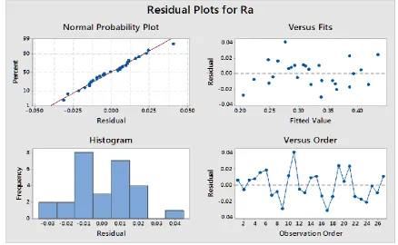
With the software Minitab 17 the statistical analysis is accrued out to estimate the affiliation of the inputs vs. output variables. Durbin Watson value in the second order equations are lies between 1to 2 which indicates that there is positive auto correlation between the predictors. Also the second order equation indicates that the predictors (input variables) explain 92.81% of the variance in the output variables. Regression models comparison for the statistical significance and the statistical values of the equations are tabulated in Table 4.1.
Table 4.1 Regression model
Regression R-sq R-sq
(adj)
R-sq (pred)
First order 90.77% 89.56% 87.35%
Second order 92.81% 89.01% 81.38%
The adjusted R - sq values are close to the R - sq values which accounts for the number of predictors in the regression model. As both the values together reveal that the model fits the data significantly. With respect to the analysis outcome, the second order regression relationship equation is taken for further evaluation and optimizing the parameters. The residual plots outcome of the statistical modeling is shown in Fig. 4.1.
362 | P a g e
Second order regression equations in terms of speed, feed and depth of cut combination is that,Ra = (0.331) – (0.000148 x Cs) + (0.79 x f) – (1.16 x DOC) – (0.000001 x Cs2) – (4.0 x f2) + (5.56 x DOC2) + (0.00100 x Cs x f) + (2.40 x f x DOC) + (0.00147 x Cs x DOC); where Cs represents the cutting speed, f denotes the feed and DOC represents the depth of cut. Through the best subset analysis result framed by Minitab software and also by analyzing the coefficients of each input parameters the feed is contributing more influence on the surface roughness comparing to the other two input variables.
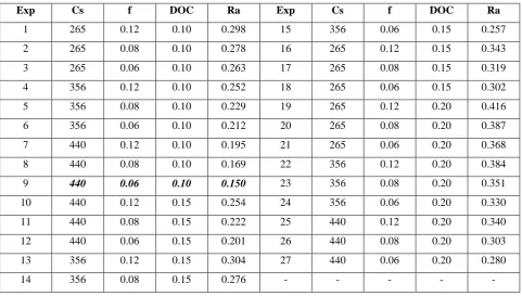
Table 4.2 Regression computed values of the surface roughness.
Exp Cs f DOC Ra Exp Cs f DOC Ra
1 265 0.12 0.10 0.298 15 356 0.06 0.15 0.257
2 265 0.08 0.10 0.278 16 265 0.12 0.15 0.343
3 265 0.06 0.10 0.263 17 265 0.08 0.15 0.319
4 356 0.12 0.10 0.252 18 265 0.06 0.15 0.302
5 356 0.08 0.10 0.229 19 265 0.12 0.20 0.416
6 356 0.06 0.10 0.212 20 265 0.08 0.20 0.387
7 440 0.12 0.10 0.195 21 265 0.06 0.20 0.368
8 440 0.08 0.10 0.169 22 356 0.12 0.20 0.384
9 440 0.06 0.10 0.150 23 356 0.08 0.20 0.351
10 440 0.12 0.15 0.254 24 356 0.06 0.20 0.330
11 440 0.08 0.15 0.222 25 440 0.12 0.20 0.340
12 440 0.06 0.15 0.201 26 440 0.08 0.20 0.303
13 356 0.12 0.15 0.304 27 440 0.06 0.20 0.280
14 356 0.08 0.15 0.276 - - - - -
The computed values for the same set of input parameters with the regression relationship is charted via Table 4.2 which reveals that theminimum surface roughness is recorded as 0.176 for the input cutting parameters combination speed 440 m / min, feed 0.06 mm / rev and depth of cut 0.10 mm.
V. OPTIMIZATION METHODOLOGIES
363 | P a g e
Table 5.1 MSE comparison of the algorithmsS No Algorithm MSE Ranking
1 Scatter Search Algorithm 0.000342549 1
2 Ant Colony Algorithm 0.000361329 2
3 Particle Swarm Optimisation 0.000361396 3
4 Genetic Algorithm 0.000678061 4
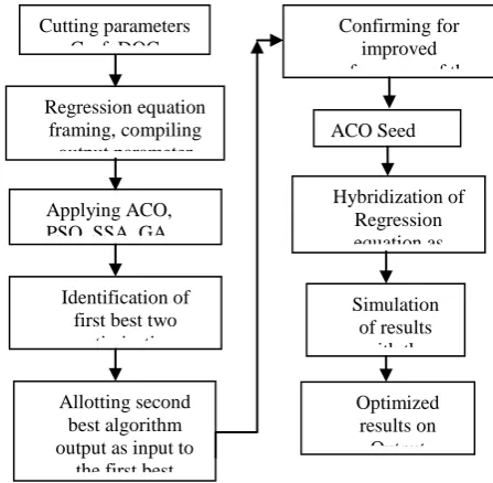
Scatter search algorithm converged with the most minimum MSE and the ACO, PSO, GA are converged subsequently with small quantity difference of MSE. As ACO is in the second place of the performance the outcome of the ACO is taken as the seed values for the first best SSA and hybridization compiling is allowed. The MSE value of this ACO seed SSA approach is resulted with the further reduced quantity 0.000254275. The convergence of the seed approach is found to be which confirms the enhanced results. The pictorial representation of the proposed method is shown in Fig. 5.1.
Figure 5.1 Block diagram of Hybridization of Regression in PSO Algorithm
Figure 5.2 MSE comparison of Algorithms Cutting parameters
Cs, f, DOC
Applying ACO, PSO, SSA, GA Optimization Regression equation
framing, compiling output parameter
values
Identification of first best two optimization algorithms
Confirming for improved performance of the
hybrid method
ACO Seed SSA
Simulation of results
with the hybrid method Optimized
results on Output parameters Allotting second
best algorithm output as input to
the first best algorithm
364 | P a g e
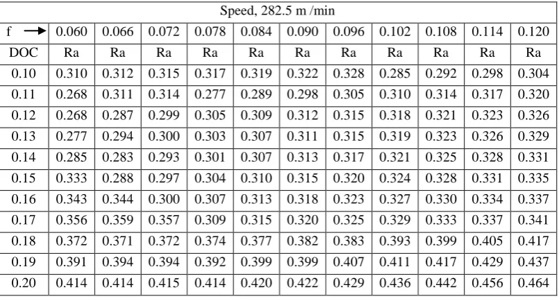
The step values given as input for simulation are as Speed = (265:17.5:440); Feed = (0.06:0.006:0.12); and Depth of cut = (0.10:0.01:0.20). The simulated results through the method adopted are marked in the Table 5.2, 5.3 and Table 5.4 for combination of speed, feed and depth of cut marked respectively.Table 5.2 Iterated values of Ra for S 265 m / min, F 0.60 – 0.120 mm / rev and DOC 0.10 – 0.20 mm
Speed, 265 m /min
f 0.060 0.066 0.072 0.078 0.084 0.090 0.096 0.102 0.108 0.114 0.120
DOC Ra Ra Ra Ra Ra Ra Ra Ra Ra Ra Ra
0.10 0.310 0.311 0.311 0.312 0.313 0.278 0.285 0.292 0.298 0.303 0.308 0.11 0.305 0.306 0.277 0.289 0.297 0.304 0.309 0.313 0.317 0.320 0.322 0.12 0.308 0.299 0.305 0.309 0.312 0.314 0.317 0.319 0.322 0.324 0.327 0.13 0.283 0.300 0.303 0.306 0.310 0.314 0.318 0.321 0.324 0.327 0.330 0.14 0.304 0.293 0.301 0.307 0.312 0.317 0.320 0.323 0.326 0.329 0.332 0.15 0.329 0.300 0.306 0.311 0.315 0.319 0.323 0.326 0.329 0.332 0.335 0.16 0.339 0.301 0.307 0.312 0.317 0.321 0.325 0.328 0.331 0.334 0.337 0.17 0.359 0.357 0.309 0.314 0.319 0.323 0.327 0.330 0.334 0.337 0.397 0.18 0.377 0.374 0.373 0.378 0.378 0.383 0.389 0.394 0.400 0.413 0.422 0.19 0.400 0.400 0.398 0.398 0.401 0.403 0.410 0.417 0.425 0.436 0.446 0.20 0.423 0.421 0.425 0.423 0.427 0.433 0.436 0.446 0.455 0.463 0.477
Table 5.3 Iterated values of Ra for S 282.5 m / min, F 0.60 – 0.120 mm / rev and DOC 0.10 – 0.20 mm
Speed, 282.5 m /min f
F
0.060 0.066 0.072 0.078 0.084 0.090 0.096 0.102 0.108 0.114 0.120
DOC Ra Ra Ra Ra Ra Ra Ra Ra Ra Ra Ra
0.10 0.310 0.312 0.315 0.317 0.319 0.322 0.328 0.285 0.292 0.298 0.304 0.11 0.268 0.311 0.314 0.277 0.289 0.298 0.305 0.310 0.314 0.317 0.320 0.12 0.268 0.287 0.299 0.305 0.309 0.312 0.315 0.318 0.321 0.323 0.326 0.13 0.277 0.294 0.300 0.303 0.307 0.311 0.315 0.319 0.323 0.326 0.329 0.14 0.285 0.283 0.293 0.301 0.307 0.313 0.317 0.321 0.325 0.328 0.331 0.15 0.333 0.288 0.297 0.304 0.310 0.315 0.320 0.324 0.328 0.331 0.335 0.16 0.343 0.344 0.300 0.307 0.313 0.318 0.323 0.327 0.330 0.334 0.337 0.17 0.356 0.359 0.357 0.309 0.315 0.320 0.325 0.329 0.333 0.337 0.341 0.18 0.372 0.371 0.372 0.374 0.377 0.382 0.383 0.393 0.399 0.405 0.417 0.19 0.391 0.394 0.394 0.392 0.399 0.399 0.407 0.411 0.417 0.429 0.437 0.20 0.414 0.414 0.415 0.414 0.420 0.422 0.429 0.436 0.442 0.456 0.464
Table 5.4 Iterated values of Ra for S 440 m / min, F 0.60 – 0.120 mm / rev and DOC 0.10 – 0.20 mm
Speed, 440 m /min f
F
0.060 0.066 0.072 0.078 0.084 0.090 0.096 0.102 0.108 0.114 0.120
DOC Ra Ra Ra Ra Ra Ra Ra Ra Ra Ra Ra
365 | P a g e
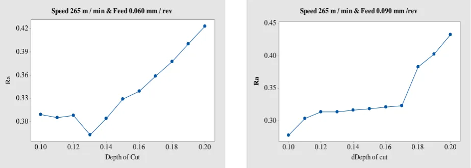
0.14 0.297 0.327 0.338 0.345 0.354 0.361 0.365 0.366 0.365 0.367 0.361 0.15 0.327 0.331 0.330 0.327 0.326 0.324 0.378 0.380 0.383 0.380 0.378 0.16 0.327 0.355 0.365 0.372 0.379 0.386 0.393 0.396 0.396 0.396 0.393 0.17 0.326 0.343 0.334 0.335 0.395 0.401 0.404 0.406 0.408 0.409 0.407 0.18 0.328 0.340 0.350 0.348 0.403 0.412 0.415 0.418 0.422 0.420 0.421 0.19 0.375 0.357 0.360 0.365 0.366 0.365 0.424 0.430 0.429 0.432 0.434The graphical representation of the surface roughness with respect to the speed 265 m / min for all combination of depth of cut and feed of 0.60 mm / rev, 0.090 mm/ rev are shown in the Fig. 5.3.
0.20 0.18 0.16 0.14 0.12 0.10 0.42 0.39 0.36 0.33 0.30
Depth of Cut
R
a
Speed 265 m / min & Feed 0.060 mm / rev
0.20 0.18 0.16 0.14 0.12 0.10 0.45 0.40 0.35 0.30
dDepth of cut
R
a
Speed 265 m / min & Feed 0.090 mm /rev
Fig. 5.3 Ra for the speed 265 m / min, feed 0.060, 0.090 mm / rev for all combination of depth of cut
The graphical representation of the surface roughness with respect to the speed 282.5 m / min for all combination of depth of cut and feed of 0.60 mm / rev, 0.090 mm/ rev are shown in the Fig. 5.4.
0.20 0.18 0.16 0.14 0.12 0.10 0.425 0.400 0.375 0.350 0.325 0.300 0.275 0.250
Depth of Cut
R
a
Speed 282.5 & Feed 0.060 mm / rev.
0.20 0.18 0.16 0.14 0.12 0.10 0.42 0.40 0.38 0.36 0.34 0.32 0.30
Depth of Cut
R
a
Speed 282.5 m / min & Feed 0.090 mm /rev
Fig. 5.4 Ra for the speed 282.5 m / min, feed 0.060, 0.090 mm / rev for all combination of depth of cut
366 | P a g e
0.20 0.18 0.16 0.14 0.12 0.10 0.38 0.36 0.34 0.32 0.30 0.28 0.26 0.24 0.22Depth of Cut
R
a
Speed 400 m / min & Feed 0.06 mm / rev.
0.20 0.18 0.16 0.14 0.12 0.10 0.46 0.44 0.42 0.40 0.38 0.36 0.34 0.32 0.30
Depth of Cut
R
a
Speed 400 m / min & Feed 0.120 mm / rev.
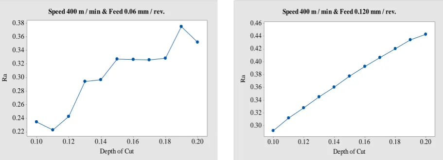
Fig. 5.5 Ra for the speed 400 m / min, feed 0.060, 0.120 mm / rev for all combination of depth of cut
VI. RESULTS AND CONCLUSIONS
Statistical significance is found to be fit for second order regression relationship between the input and output parameters. The best subset analysis and the coefficients of each input parameters reveals that the feed is contributing more influence on the surface roughness comparing to the other two input variables. Out of SSA, ACO, PSO, GA optimisation algorithms the SSA converges towards the accuracy level in computation. ACO seed SSA algorithm hybridization with regression relationship as input converges with further minimum mean error. The optimised result for this experiment is tabulated in Table 6.1.
Table 6.1 Optimised results
S F DOC Optimised Ra
440
0.06
0.11
0.223
The proposed hybridization method may be considered for future references while compiling the optimisation of parameters in other process also. Manufacturers may use this as a referenceset for their processing in order to select the optimal parameter combination according to the required surface finish value to avoid the rework and part rejection. The analysis can be extended to find out the tool wear, material removal rate, machining time, power consumption etc. The computed values of the regression relationship equations need to be examined and ensured for statistical significance in all aspects while assigning as the input values for compiling. By selecting the steps value much closer leads to get smoother curve fittings for references. The presentation in graphs may be taken as a ready reckoner by the manufacturers for processing the parts. Attempts may be exercised with other familiar accepted optimisation algorithms.
REFERENCES
[1] Maciej Grzenda & Andres Bustillo, 2013, “The evolutionary development of roughness prediction models”, Applied
Soft Computing, vol. 13, no. 5, pp. 2913-2922.
[2] Azlan Mohd Zain , Habibollah Haron & Safian Sharif, 2010, “Application of GA to optimize cutting conditions for minimizing surface roughness in end milling machining process”, Expert Systems with Applications, vol. 37, pp. 4650-4659.
[3] Muthukrishnan. N, Murugan. M, Prahlada Rao. K. 2008. Machinability issues in turning of AlSiC(10p) metal matrix
367 | P a g e
[4] Oezel.T, Karpat. Y. 2005. Predictive modeling of surface roughness and tool wear in hard turning using regressionand neural networks. Int J Mach Tools Manuf. 45, 467-479.
[5] Tekiner. Z, Yesilyurt. S. 2004. Investigation of the cutting parameters depending on process sound during turning of
AISI 304 austenitic stainless steel. Mater Des. 25, 507-513.
[6] Nikolaos, Galanis, E. Dimitrios and Manolakos, Surface roughness prediction in turning of femoral head, Int J Adv
Manuf Technol, 51, 2010, 79-86.
[7] Hascalik, A. & Caydas, U (2007). Optimization of turning parameters for surface roughness and tool life based on
the Taguchi method. Int. J. Adv. Manuf. Tech, pp.1147-1154.
[8] Suresh, P.V.S, Rao, P.V, Deshmukh, S.G, 2002, A genetic algorithmic approach for optimization of surface
roughness prediction model, International Journal of Machine Tool and Manufacture, vol. 42, pp. 675-680.
[9] Tzeng, Y.F, Chen, F.C, 2006, Multi-objective process optimization for turning of tool steels, International Journal