A FRAMEWORK FOR APPLYING SURROGATE SAFETY MEASURES FOR SIDESWIPE CONFLICTS

A FRAMEWORK FOR APPLYING SURROGATE SAFETY MEASURES

FOR SIDESWIPE CONFLICTS

Hamid Behbahani1_{, Navid Nadimi}21

1, 2 _{Iran University of Science and Technology, Department of Civil Engineering, Iran}

Received 10 December 2014; accepted 11 February 2015

Abstract:Surrogate safety measures (SSM) as indicators of accidents are useful tools in safety evaluations. Nowadays, developing intelligent vehicles without drivers in order to reduce the human errors is a popular topic in civil engineering. Such vehicles are equipped with intelligent collision avoidance systems (CAS), in which safety indicators are applied as warning strategies. Heretofore, different safety indicators have been developed, but most of them are suitable for rear-end conflicts. In this paper, a new framework is proposed to calculate the risk of sideswipe collisions at each instant based on SSM. For this purpose, time-to-collision (TTC) and post-encroachment time (PET), as the most important time-based indicators would be applied and a new method would be presented to calculate these indicators. The application of the framework is illustrated by microscopic traffic data for an arterial road. In all, the new framework has three main applications: 1- As a warning strategy for CAS, 2- Specifying dangerous positions and 3- Identifying aggressive drivers.

Keywords:time-to-collision, safety, modeling, highways.

2 _{Corresponding author: [email protected]}

1. Introduction

There are three main approaches for safety estimations: 1- Using crash frequency or crash rates over a short-term or long-term period, 2- Indirect safety measures and 3- Statistical analysis technique. Indirect safety measures refer to traffic conflict technique (TCT), which does not need crash data for analysis (HSM, 2010). Because of the difficulties to collect crash data due to the lack of detailed and comprehensive data, TCT has become popular for safety analysis in recent years. TCT first has been formally applied by Perkins and Harris (1967) in General Motors Corporation. Their approach was to observe and count situations in which vehicles take evasive maneuvers to avoid collision. However, this procedure

was difficult and imprecise because of the human errors and limitations (Chind and Quek, 1997). Therefore, gradually objective methods replaced, which depend on surrogate safety measures (SSM). SSM are indicators of evasive maneuvers and if being defined properly are suitable tools to detect dangerous situations (Barcelo et al., 2003; Archer, 2005; Gettman and Head, 2003; Craveiro Cunto, 2008; Garber and Gousios, 2009; Sobhani et al., 2013; Young et al., 2014). SSM have been developed for two main purposes: 1- Calculating the probability of a collision occurrence (collision risk) and 2- Calculating the outcomes of a potential collision (collision severity).

driver. Such vehicles must be equipped with collision avoidance systems (CAS) which can detect any collision risk. A warning strategy must be defined for CAS to detect any collision risk soon enough to apply a proper reaction. SSM as indicators of accidents are suitable for this purpose (Saffarzadeh et al., 2013).

Heretofore, various SSM have been developed for different types of facilities and conflicts, but most of them are suitable to determine rear-end collision risk. In literature, there is no clear methodology to determine the risk of sideswipe collisions by indirect methods. Also in the calculation of SSM, motion characteristics of vehicles are usually neglected. Therefore, in this paper a new framework is developed to calculate the sideswipe collision risk, based on the motion characteristics of vehicles.

2. Literature Review

In this section, first SSM are reviewed and then the recent developments in the calculation of one of the most important time based indicators, namely time-to-collision (TTC) will be observed.

2.1. Surrogate Safety Measures

• Time-To-Collision (TTC)

TTC first was defined by Hayward (1971) as the time that remains until a collision occurrence between two vehicles if the collision course and speed difference are maintained constant (Hayward, 1971). When TTC is small, there is an imminent danger of collision (Vogel, 2003). TTC for rear-end conflicts can be calculated by Eq. (1) (Minderhoud and Bovy, 2001).

( ) ( )

( ) ( ) ( )

( ) ( )

L F L

F F L

F L

X t X t l

TTC t X t X t

X t X t

− −

= ∀ >

−  

 

(1)

Where;

TTC: Time-to-collision,

X : Vehicle position (L: leading and F: following),

X_{: Vehicle speed (L: leading and F:}

following), l: Vehicle length.

• Post Encroachment Time (PET)

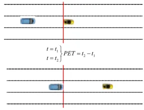
PET is the difference between times that a vehicle enters a conflict point until another vehicle arrives to this point (Cooper, 1983).

When PET is small; there is a potential danger of collision (Vogel, 2003). Fig. 1 displays the procedure for calculating PET in a highway.

1

2 1

2

t t

PET t t t t

=  _{= −}  = 

Fig. 1.

Post Encroachment Time (PET) in a Highway

• Deceleration Rate to Avoid Collision (DRAC)

2

, ,

, ,

( )

2 ( )

F t L t

t

L t F t L

X X

DRAC

X X l

− =

− −

 

 

 

(2)

• Proportion of Stopping Distance (PSD)

The PSD is the ratio of distance that is available between two vehicles and the distance, which is required to avoid a collision with the maximum available deceleration rate (MADR) (Brian et al., 1978).

, ,

2 F,

( )

( ₂ )

L t F t L t

X X l

PSD X

MADR

− −

= _{ (3)}

• Crash Potential Index (CPI)

Crash potential index, is the probability that the deceleration rate to avoid a collision (DR AC) exceeds MADR, at a moment. MADR depends on the vehicle type and some environmental conditions like pavement skid resistance. CPI is presented by Eq. (4) (Craveiro Cunto, 2008).

,

( ). .

i

i

tf

i t t ti

i

i

P DRAC MADR t b

CPI

T =

≥ ∆

=

∑

Where;

i

CPI : Crash potential index for subject vehicle i,

t

∆ : Time step,

i

T: Total travel time,

i

ti and tfi: Initial and final time steps.

The parameter b in the above equation denotes a binary state variable, 1 if a vehicle interaction exists and 0 otherwise.

• Unsafe Density (UD)

UD tries to consider the severity of a potential crash if the leading vehicle decelerates with maximum braking capacity. Assuming a collision has occurred in a car-following situation then (Barcelo et al., 2003):

max

(X

). .

/

0

0

L F F d

d

UD

X

X R

b b

if b

R

else

=

−

<















(5)

Where;

b: Deceleration rate of leading vehicle, bmax: Maximum possible deceleration rate

of leading vehicle.

• Max Speed (MaxS)

It is the maximum speed of vehicles involved in the conflict. MaxS is an effective measure to consider the severity of the collision (Gettman and Head, 2003).

Relative Speed (∆v₎

v

∆

in the conflict. In addition, this measure is for reflecting the collision severity (Gettman et al., 2003).

• Kinetic Energy

From Newtonian physics, we know that a moving vehicle has a kinetic energy as Eq. (6) (Sobhani et al., 2011):

2

1

2 s s

Where;

K: Kinetic energy,

s

m: Mass of the subject vehicle and

s

X _{: Speed of the subject vehicle.}

When the subject vehicle collides with another vehicle, the kinetic energy will reduce and changes to heat and deformation in the vehicle. The kinetic energy transferred to the subject vehicle is (Sobhani et al., 2011):

2

1 2

s s s

KE = m X∆ ₍₇₎

Where;

s

KE : Kinetic energy transferred to the subject vehicle and

s

X

∆ _{: Speed change of the subject vehicle}

before and after the collision.

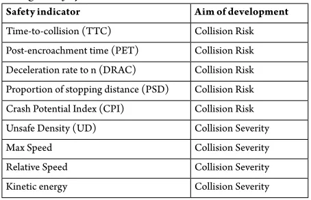
In Table 1 a summarized review of the SSM is presented.

Table 1

Surrogate Safety Measures Review

Safety indicator Aim of development Time-to-collision (TTC) Collision Risk Post-encroachment time (PET) Collision Risk Deceleration rate to n (DRAC) Collision Risk Proportion of stopping distance (PSD) Collision Risk Crash Potential Index (CPI) Collision Risk Unsafe Density (UD) Collision Severity Max Speed Collision Severity Relative Speed Collision Severity Kinetic energy Collision Severity

2.2. TTC Improvements

There has been two major limitations in the conventional definition of TTC, 1- Vehicles continue with constant speed until collision occurrence, 2- Being suitable for rear-end conflicts. To resolve these disadvantages, Saffarzadeh et al. (2013) proposed a general formulation for TTC, which considers the motion characteristics of vehicles until collision occurrence and Laurshyn et al. (2010) developed a new method to calculate TTC for different angles of collision (Saffarzadeh et al., 2013; Laurshyn et al., 2010).

• General Formulation for Time-To-Collision (GTTC)

Saffarzadeh et al. (2013) considered motion characteristics, being variable in the TTC calculation process.

They suggested a theoretical formulation to calculate TTC, if assuming that the (k)

th derivative of position being constant.

0 1 0 1 1 ! 1,2,3,... 1 ! n k n F

F F n

n n k

n L

L L n

n

X

X X _{n t} t

k X

X X t

n t = =  _{= +}  _×∂ _×    _∂     ₌   ∂   _{= + × ×}    _{ ∂ }  ∑

∑ (8)

Where; n n X t ∂

∂ : nth derivative of X , for instance

3

3F F

X _X

t

∂ ₌

∂ 

0F

X : The initial position of the following vehicle,

0L

X : The initial position of the leading vehicle.

Eq. (9) has been defined as the necessary and sufficient condition for rear-end collision:

0

F L L

X −X + = ⇔l rear-end collision (9)

Replacing Eq. (8) into Eq. (9), results in kth

degree polynomial whose solution is TTC:

0 0 1 1 ₀ ! n n k n F L

F L L n n

n

X X

X X L t

n t t

=  ∂ ∂   − + +  × _∂ − _∂ × =     ∑ (10)

TTC is the minimum, non-zero and real (non-complex) solution of Eq. (10), (for t).

• Time-To-Collision for a Moving Line Section and a Point

Laureshyn et al. (2010) suggested calculating TTC between two vehicles at any angle that they might have a collision. They stated that in any possible collision, a corner of one of the vehicles touches one side of the other one. Therefore, a new concept for TTC has been developed which calculates TTC between a moving line section and a point (Laurshyn et al., 2010).

Consider a line section named “ab”, with (r₁, s₁) and (r₂, s₂) as the initial coordinates of its end points and a point named “p”, with current coordinates (r₃, s₃). Based on equations of motion the position of point “p”, t seconds later is:

3

3

p pX

p pY

x r X t

y s X t

 = +   = +    (11) Where; pX

X



direction,

pY

X



direction.

The same as Eq. (11), the coordinates of line section end points, t seconds later would be:

1 2

1 2

a abX b abX

a abY b abY

x r X t x r X t

a and b

y s X t y s X t

 = +  = +     = + = +      

  (12)

Where;

abX

X



direction,

abY

X



direction.

The line equation in canonical form with k as line slop is:

1

1 y s

x r k

−

− = ₍₁₃₎

TTC would be calculated if replacing point coordinates (Eq. (11)) in line equation:

3 1 3 1

( ) ( )

( ) ( )

collision

abY pY abX pX

s s k r r t

X X k X X

− − −

=

− − −

Here only positive values of

t

t

TTC, like Eq. (15).

( ) ( ) ( )

( ) ( ) ( )

a coll p coll b coll

a coll p coll b coll

x t x t x t

y t y t y t

≤ ≤



 _{≤ ≤}

 (15)

3. Methodology

Various SSM have been developed to determine the collision risk, but most of them are suitable for rear-end conflicts. Therefore, there are some problems in the process of calculating sideswipe collision risk:

1. It is not clear which safety indicator must be applied at each instant to calculate the sideswipe collision risk.

2. Improvements which have been suggested by Saffarzadeh et al. (2013) and Laurshyn et al. (2010) are merely for TTC. Now it is not clear, how other SSM must be improved in order to consider the motion characteristics.

3. The procedure illustrated by Laurshyn et al. (2010) to calculate TTC for different angles is challenging. In their method, the motion of both vehicles has been considered to be constant speed. In addition, the parameters such as the coordinates of two points of the subject vehicle, slope of the subject and the bullet vehicle in relation to the horizontal axis are needed at each instant to calculate TTC.

Table 1 indicates that TTC, PET, DRAC, CPI and PSD are suitable to determine the collision risk and KE, UD, Max speed and Relative speed are proper for determining the outcomes of a potential collision (collision severity). This paper concentrates just on the first group and tries to present a framework to determine the risk of sideswipe collisions.

Investigations show that DRAC, the CPI and PSD cannot be helpful to determine the sideswipe collision risk. Because unlike the rear-end and head-on conflicts, in sideswipe conflicts, it is not necessary for vehicles to decelerate to speeds near zero (the main condition in developing DRAC, PSD and CPI).

Here even slight changes in the speed of each vehicle can help avoiding the collision. In addition, DRAC, CPI and PSD, only consider the specifications of one vehicle while TTC and PET consider the motion characteristics of a pair of vehicles simultaneously. Thus, just PET and TTC are selected for calculating the risk of sideswipe collisions.

0 0

X r

Y p

=   = 

α

0

0 0 0 X a

Y

=   = 

b Subject Vehicle

Vehicle ID: a

Bullet Vehicle Vehicle ID: b

Fig. 2.

A General Scenario for Sideswipe Collision

Based on the motion equations, t seconds later the position of each vehicle can be presented by Eq. (16), if considering the kth

time derivative of position being constant.

1 1

1 1

1 1

0 _{! !}

, b

1 1

0 _{! !}

n n

k k

n n

a b

a n b n

n n

n n

k k

n n

a b

a n b n

n n

x x

x _{n t} t x r _{n t} t a

y y

y _{n t} t y p _{n t} t

= =

= =

  ∂    ∂ 

= + × × = + × ×

  _∂    _∂ 

     

 

 ∂   ∂ 

 _{= + × ×}  _{= + × ×}

   

  ∂    ∂ 

 

∑ ∑

∑ ∑ (16)

At the collision point, the horizontal and vertical coordinates of both vehicles must be the same. So, we put X_a = X_b and Y_a = Y_b, solving each equation two values will be achieved like t₁ and t₂ as the solution of these equations. Now one of these cases might happen: t₁ &t₂ ≥ 0, t₁ &t₂ < 0, t₁ ≥ 0 &

t₂ < 0 and t₁ < 0&t₂ ≥ 0. Since the subject vehicle moves on the horizontal axis, thus the vertical coordinate of the collision point is always zero (Y_a = Y_b = 0), this means that

to have a collision point, Y_a = Y_b must have a solution or t₂ ≥ 0. Also, in order to have a collision the position of the bullet vehicle at t₂ must be geater or equal to zero (X_b t₂) ≥ 0 ), because the initial position of the subject vehicle is (0,0) and it moves forward. These conditions are the necessary and sufficient conditions to have a collision point in sideswipe conflicts.

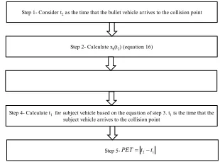
3.1. PET Calculation

PET refers to the time difference that the first vehicle passing the collision point, until the second one arrives. In order to calculate PET, first it should be checked if vehicles have a collision point as described in the previous section. Then the algorithm presented in Fig. 3, would be applied to calculate PET.

Step 1- Consider t2as the time that the bullet vehicle arrives to the collision point

Step 2- Calculate xb(t2) (equation 16)

Step 4- Calculate t1for subject vehicle based on the equation of step 3. t1is the time that the

subject vehicle arrives to the collision point

Step 5-PET t t=2−1

Step 3- put xa(t1)=xb(t2)

Fig. 3.

3.2. TTC Calculation

TTC refers to the time remaining to a potential collision. Assume that the subject and the bullet vehicles have a collision point. If t₁ = t₂ then it means that in t = t₁ = t₂ seconds later horizontal and vertical coordinates of both vehicles would be the same therefore TTC= t₁ = t₂and PET = 0. If t₁ ≠ t₂ then TTC cannot be defined at that moment and just we have a collision point.

3.3. Calculating the Sideswipe Collision

Risk

Now there is a question, which indicator must be applied to determine the sideswipe collision risk, TTC or PET? To answer this question, it should be reminded that TTC refers to the imminent danger, but PET implies the potential danger. Based on this statement, safety analysis will be done in two layers, TTC in the first and PET in the second layer. The first layer is called RED risk and the second one is YELLOW risk. In fact, at each instant, first TTC must be calculated. When TTC is computable, then the sideswipe collision risk is RED. Nevertheless PET must be calculated and the risk is YELLOW. Now a method is necessary to calculate the value of RED and YELLOW risks.

To have a better comparison between TTC values at each moment, a mapping function is needed, which gives a value in the range of [0,1] instead of TTC. We know that the collision risk increases when TTC decreases and the risk is expected to have an exponential increase, when TTC is decreasing. Also literature review indicates that, TTC values more than 5 seconds are safe (Hirst and Graham, 1997; Hogema and

Janssen, 1996; Van der Horst, 1990). Based on these conditions, Eq. (17) is proposed to calculate the “RED” risk.

exp 0 5 sec

0 5

TTC R

R

SSCR TTC

SSCR TTC

−

 = ∀ ≤ <

 

= ∀ >

 (17)

Where;

SSCRR: RED Sideswipe collision risk.

When TTC cannot be computed and just PET is available, a virtual TTC would be defined and named TTC'. TTC'would be considered as the minimum (t1, t2) if t1, t2 ≥

0. Now again SSCRR an be computed with

Eq. (17). However TTC' is virtual, since vehicles do not reach to the collision point at the same time and there is a time difference like PET. Whatever the PET value is greater then it means that the difference between t1

and t2 is more and the probability of having

a real TTC is less. This relationship is also expected to be exponential. Eq. (18) would be applied to calculate the “YELLOW” sideswipe collision risk.

1

( ).

Y R PET

SSCR SSCR TTC

e ′

= (18)

When t or t1 2<0, SSCRY =0. This procedure is applied as a preliminary method and it should be improved in future research.

For a time interval like T, the overall value of sideswipe collision risk would be determined by Eq. (19).

0 0

(T) T ( ) T ( )

i R Y

t t

SSCR SSCR t SSCR t

= =

=

∑

∑

Where;

(T)

i

4. Applying the New Framework

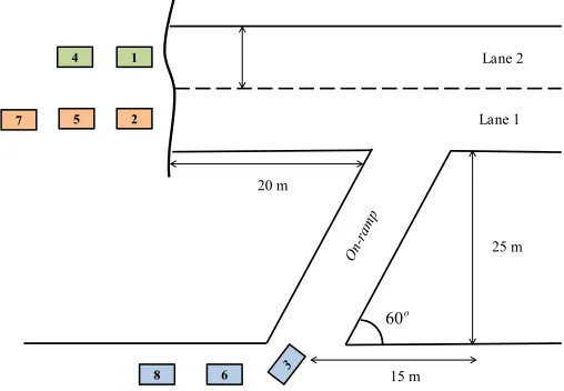
In order to calculate SSCR, microscopic traffic data are necessary. Here we have the traffic stream in a section of a freeway in Tehran, capital of Iran with an on-ramp entering an arterial road with no deceleration

lane. The section under study has two lanes and during the study period, eight vehicles have entered the section.

There is no lane-change, but lanes are wide enough that two vehicles can move beside each other. Fig. 4 displays this section.

20 m

25 m

15 m

1 4

7 5 2

8 6

Lane 2

Lane 1

60o

3.6m

Fig. 4.

Characteristics the Section under Study

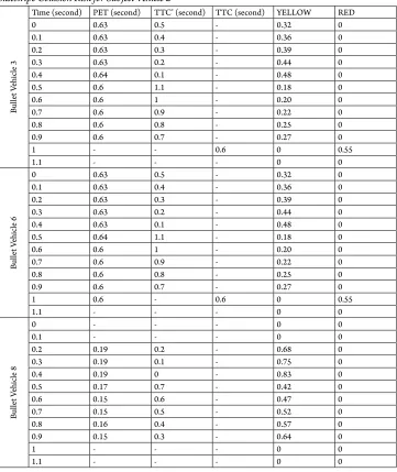
Based on the proposed framework, the RED and YELLOW sideswipe collision risk can be calculated for each vehicle. Here subject vehicles are 2, 5 and 7 and bullet vehicles are 3, 6 and 8. Vehicles 1 and 4 have no sideswipe collision risk. The results for subject vehicle 2 is presented in Table 2 as an example.

However, in Figs. 5-7, the summarized results can be observed for each subject vehicle.

0.00 0.10 0.20 0.30 0.40 0.50 0.60 0.70 0.80 0.90

0 0.1 0.2 0.3 0.4 0.5 0.6 0.7 0.8 0.9 1 1.1

C

ollis

io

n R

is

k

Time (Second)

YELLOW RED TOTAL

Fig. 5.

The Variations of Sideswipe Collision Risk During Study Period, Subject Vehicle 2

0.00 0.20 0.40 0.60 0.80 1.00 1.20 1.40

0.2 0.3 0.4 0.5 0.6 0.7 0.8 0.9 1 1.1 1.2 1.3

C

ollis

io

n R

is

k

Time (Second)

YELLOW RED TOTAL

Fig. 6.

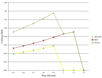
The Variations of Sideswipe Collision Risk During Study Period, Subject Vehicle 5

0.00 0.20 0.40 0.60 0.80 1.00 1.20 1.40 1.60

0.5 0.6 0.7 0.8 0.9 1 1.1 1.2

C

ollis

io

n R

is

k

Time (Second)

YELLOW RED TOTAL

Fig. 7.

Table 2

Sideswipe Collision Risk for Subject Vehicle 2

Bul

le

t V

ehicle 3

Time (second) PET (second) TTC’ (second) TTC (second) YELLOW RED

0 0.63 0.5 - 0.32 0

0.1 0.63 0.4 - 0.36 0

0.2 0.63 0.3 - 0.39 0

0.3 0.63 0.2 - 0.44 0

0.4 0.64 0.1 - 0.48 0

0.5 0.6 1.1 - 0.18 0

0.6 0.6 1 - 0.20 0

0.7 0.6 0.9 - 0.22 0

0.8 0.6 0.8 - 0.25 0

0.9 0.6 0.7 - 0.27 0

1 - - 0.6 0 0.55

1.1 - - - 0 0

Bul

le

t V

ehicle 6

0 0.63 0.5 - 0.32 0

0.1 0.63 0.4 - 0.36 0

0.2 0.63 0.3 - 0.39 0

0.3 0.63 0.2 - 0.44 0

0.4 0.63 0.1 - 0.48 0

0.5 0.64 1.1 - 0.18 0

0.6 0.6 1 - 0.20 0

0.7 0.6 0.9 - 0.22 0

0.8 0.6 0.8 - 0.25 0

0.9 0.6 0.7 - 0.27 0

1 0.6 - 0.6 0 0.55

1.1 - - - 0 0

Bul

le

t V

ehicle 8

0 - - - 0 0

0.1 - - - 0 0

0.2 0.19 0.2 - 0.68 0

0.3 0.19 0.1 - 0.75 0

0.4 0.19 0 - 0.83 0

0.5 0.17 0.7 - 0.42 0

0.6 0.15 0.6 - 0.47 0

0.7 0.15 0.5 - 0.52 0

0.8 0.16 0.4 - 0.57 0

0.9 0.15 0.3 - 0.64 0

1 - - - 0 0

1.1 - - - 0 0

5. Conclusion

Traffic conflict technique with the help of SSM can be applied as an indirect method for safety evaluations. Most of the SSM are

For this purpose first most important SSM are reviewed. Then TTC and PET as time-based indicators are selected for calculating the sideswipe collision risk. TTC referrers to an imminent danger and PET implies the potential danger. TTC and PET that are introcuced in the literature do not consider the motion characterstics of vehicles and also are not defined for angular conflicts. Therefore, new calculation methods are presented for PET and TTC for angular conflicts by considering motion characteristics of vehicles. Then the collision risk is divided into two categories, which are named YELLOW and RED risk. YELLOW and RED risks deal with PET and TTC values respectively. RED risk has a priority in comparison to YELLOW. The results obtained from this framework can have various applications: 1- Different defensive strategies can be defined for CAS, based on the value of YELLOW and RED risks in order to have a proper reaction automatically. 2- Dangerous positions, e.g. a point with a poor geometric design that leads to accidents can be detected just by data collected in several hours or days. 3- Aggressive drivers, which drive risky, can be identified based on the values of YELLOW and RED risks, obtained from video cameras.

References

Archer, J. 2005. Indicators for traffic safety assessment and prediction and their application in micro-simulation modelling: A study of urban and suburban intersections. Unpublished Ph.D. thesis, Royal Institute of Technology, Stockholm, Sweden.

Barcelo, J.; Montero, L.; Perarnau, J.; Torday, A. 2003. Safety indicators for micro-simulation based assessments. In 82nd Annual meeting of the Transportation Research Board, Washington, D.C., USA.

Brian, L.; Allen, B.; Shin, T.; Cooper, P.J. 1978. Analysis of traffic conflicts and collisions, Transportation Research Record: Journal of the Transportation Research Board, 667: 67-74.

Chin, H.C.; Quek, S.T. 1997. Measurement of Traffic Conflicts, Safety Science. DOI: http://dx.doi.org/10.1016/ S0925-7535(97)00041-6, 26(3): 169-185.

Cooper, P.J. 1983. Experience with traffic conflicts in Canada with emphasis on “post encroachment time” techniques. In Proceedings of the NATO Advanced Research Workshop on International Calibration Study of Traffic Conflict Technique.

Craveiro Cunto, F.J. 2008. Assessing Safety Performance of Transportation Systems using Microscopic Simulation. Unpublished Ph.D. thesis, Dept. of Civil Engineering, Waterloo, Canada.

Garber, N.J.; Gousios, S. 2009. Relationship between Time to Collision Conflicts and Crashes on Interstate Highways Subjected to Truck Lane Restrictions. In

88th Annual Meeting of the Transportation Research Board. Washington, D.C. 15 p.

Gettman, D.; Head, L. 2003. Surrogate safety measures from traffic simulation models. Technical report, Federal Highway Administration - FHWA.

Hayward, J. 1971. Near misses as a measure of safety at urban intersections. Unpublished Ph.D. thesis, Dept. of Civil Engineering, The Pennsylvania State Univ., University Park, PA.

Highway Safety Manual. 2010. American Association of State Highways and Transportation Officials, 1st Edition.

Hogema, J.H.; Janssen, W.H. 1996. Effects of intelligent cruise control on driving behavior. Soesterberg, the Netherlands, TNO Human Factors, Report TM-1996-C-12.

Laureshyn, A.; Svensson, A.; Hyden, Ch. 2010. Evaluation of traffic safety, based on micro-level behavioral data: Theoretical framework and first implementation, Accident Analysis and Prevention. DOI: http://dx.doi.org/10.1016/j.aap.2010.03.021, 42(6): 1637-1646.

Minderhoud, M.M.; Bovy, P.H.L. 2001. Extended time-to-collision measures for road traffic safety assessment,

Accident Analysis and Prevention. DOI: http://dx.doi. org/10.1016/S0001-4575(00)00019-1, 33(1): 89-97.

Perk ins, S.; Harris, J. 1967. Traffic conf lict characteristics accident potential at intersections,

Highway Research Board, 225: 35-43.

Saffarzadeh, M.; Nadimi, N.; Nasealavi, S.; Mamdoohi, A.R. 2013. A general formulation for time to collision. In Proceedings of the ICE Transport, 166: 294-304.

Sobhani, A.; Young, W.; Bahrololoom, S.; Sarvi, M.; 2013. Calculating Time-To-Collision for Analyzing Right Turning Behavior at Signalized Intersections,

Road and Transport Research, 22(3): 49-61.

Sobhani, A.; Young, W.; Logan, D.; Bahrololoom, S. 2011. A kinetic energy model of two-vehicle crash injury severity, Accident Analysis and Prevention. DOI: http:// dx.doi.org/10.1016/j.aap.2010.10.021, 43(3): 741-754.

Van der Horst, A. 1990. A Time-Based Analysis of Road User Behavior in Normal and Critical Encounters. TNO Institute for Perception, Soesterberg, Netherlands.

Vogel, K. 2003. A comparison of headway and time to collision as safety indicators, Accident Analysis and Prevention. DOI: http://dx.doi.org/10.1016/S0001-4575(02)00022-2, 35(3): 427-433.