Ionospheric Tomography by Neural Network Collocation Method
Tatsuoki TAKEDA and XiaoFeng MA
1)The University of Electro-Communications, Chofu 182-8585, Japan
1)Xilisoft Corporation, Haiden District, Beijing 100080, China (Received 2 December 2006/Accepted 19 July 2007)
We describe a neural network collocation method (NNCM) for tomographic image reconstruction with small amount of projection data, which has been successfully applied to the three-dimensional ionospheric tomography based on the dataset of signal delays from the GPS satellites. In NNCM the neural network is trained by mini-mizing an object function composed of squared residuals of the governing equations evaluated at the collocation points and some constraining conditions imposed usually by observation data. This method is applied not only to the computerized tomography but also to the analyses of various inverse problems such as the data assimilation, the parameter estimation, the time series prediction, and so on.
c
2007 The Japan Society of Plasma Science and Nuclear Fusion Research
Keywords: ionospheric tomography, multilayer neural network, neural network collocation method, residual minimization training
DOI: 10.1585/pfr.2.S1015
1. Introduction
In this paper we describe that the “neural network with residual minimization training (NNRMT)” [1] used for the neural network collocation method (NNCM) can be applied to the tomographic image reconstruction with small amount of projection data [2]. As a typical example of such a problem it has been successfully applied to the three-dimensional computerized ionospheric tomography (CIT) [3].
1.1
Computerized ionospheric tomography
Reconstruction of ionospheric electron density profile based on measurements of radio signals from navigation satellites has become an important technique for various applications ranging from academic to practical purposes. As the ionospheric total electron content (TEC) is an in-tegrated value of the ionospheric electron density along a ray path of the radio signal from a satellite to a ground receiver, the problem to reconstruct the electron density profile from a set of the TEC values is a kind of comput-erized tomography (CT). Since Austen et al., [4] applied the algebraic reconstruction technique (ART) to the two-dimensional analysis of model TEC data generated by a computer simulation various methods for CIT were pro-posed and applied to analyses of model data and real obser-vation data. Though the two-dimensional ionospheric to-mography has been studied extensively from both the the-oretical and observational aspects [5–7], in these studies only the ionospheric structure within a cross-section de-fined by the satellite orbit and the ground receiver array can be obtained, which limits strongly the observation time and place. In order to cope with the problem methods for
author’s e-mail: [email protected]
the three-dimensional CIT are being studied intensively by many authors [8–14]. In these analyses, usually, TEC data obtained for the ray paths between the Global Positioning System (GPS) satellites and ground receivers are used and to attain higher resolution sometimes the occultation mea-surement by the Low Earth Orbit (LEO) satellite is incor-porated. The vertical density profiles are often expressed by function series based on the empirical orthogonal func-tions (EOF) derived from the international reference iono-sphere (IRI) model. By using the GPS-ground receiver sys-tem many ray paths in a three-dimensional domain become available and the occultation measurement makes up scant information on the vertical density profile. The problems on the scarcity of the ray paths and the lack of the near-horizontal ray paths, however, are not solved sufficiently by these methods. To solve these problems we proposed a new CT analysis method effective for the case of small amount of projection data based on NNCM and success-fully applied it to the three-dimensional CIT by using data of the GPS Earth Observation Network (GEONET) [15] and the ionosonde data.
1.2
Neural network with residual
minimiza-tion training
A neural network is composed of many neurons with simple processing ability. A neuron has some input chan-nels and one output channel. A weight value is assigned to each input channel including a bias channel and weighted sum of the input data is nonlinearly transformed by an activation function. We consider a multilayer network in which neurons are aligned in layers as an input layer, hid-den layer(s), and an output layer. We skip details of the multilayer neural network as these are described by many authors (e.g., [16, 17]).
c
2007 The Japan Society of Plasma
Usually the multi-layer neural network is trained for a set of combinations of an input dataset (a “pattern”) and a known output dataset (a “teacher dataset”) by minimizing an object function (a sum of squared differences of output data from the teacher data) with respect to the internal pa-rameters (weights) of the neural network. The training is carried out by the commonly used error back-propagation method [18]. It should be noted that for the sake of expla-nation of the learning process we have hitherto described the conventional learning process where teacher data are necessary but in the case of NNRMT teacher data are not necessary. In the NNCM method values of the independent variables (the position of the collocation points) of the out-put variable (the solution of the problem) are fed and the weights of the neural network are determined so that the sum of the squared residuals are minimized. This is a map-ping from a collocation point to the functional value under the condition that the governing equation is satisfied by the solution.
For our purpose the following features of the multi-layer neural network are very important.
(1) It can approximate any functions within any preci-sion under a certain mathematical condition [19, 20]. Though this existence theorem does not guarantee that the solution could be attainable, an approximate solution is often attainable comparatively easily prob-ably because the multi-layer neural network repre-sents a function expansion by “variable basis func-tions” instead of “fixed basis funcfunc-tions” such as the system of orthogonal functions (as the trigonometric functions).
(2) Generalization property is controlled by selecting the network structure and iteration number appropriately, and the method is robust against noises in input data. These are empirically believed though reliable gen-eral recipes for obtaining a result with the minimum approximation error have not been found despite of extensive theoretical works. As the interpolation and smoothing functions are inherently included in the multi-layer neural network [21] the difficulty in CT that arises from an imperfect set of projection data is relaxed considerably by using the neural network. (3) Wide range of complex nonlinear problems can be
solved by selecting the object function appropriately because the learning process is a nonlinear optimiza-tion of an object funcoptimiza-tion composed of the above de-scribed flexible “approximate functions”, their deriva-tives, and integrals.
2. Computerized Tomography by Neural
Network Collocation Method
We assume to inject a beam represented by a quan-tity (beam quanquan-tity) qp()=0into the object along the p-th projection path whereis the coordinate along the path and the quantity is measured after the beam goes out from the
object at=L. The change of the beam quantity dqp() is assumed to depends on the local value of the beam quantity and the target quantity distribution (ρ(r)) as
dqp=f
ρ(r),qp
d. (1)
When we are to reconstruct the electron density distribu-tion N(r) in a plasma by measuring the phase delayφpof the injected electromagnetic wave the above beam quan-tity qpis the phase delayφpand the target quantityρ(r) is the electron density distribution N(r). In this case the inte-grand of the above integral does not depend on the phase delayφpbut depends on the electron density N(r) linearly, and the following equation is derived.
∆φp≡φp(L)−φp(0)=A
=L(p)
=0
N(r)d, (2)
where A is a constant and (p) denotes the p-th integra-tion path. In this analysis we use a neural network sys-tem shown in Fig. 1, where a neural network represents the electron density distribution as a function of the spatial po-sition. If the coordinate values of a spatial position are fed to the input channel the electron density at the given posi-tion is obtained from the output channel. Therefore, if we prepare numerical integration points (collocation points: u = 1,. . . U) on the p-th projection path (x(p)u = ru) be-forehand the electron densities at the integration points ((u)p =N(x
(p)
u )) are calculated and the corresponding phase delay for the p-th projection path∆φNN
p is obtained. The object function is, therefore, defined as
E=1
2 P
p=1
∆φNN p −∆φ
meas p
2
, (3)
∆φNN p =A
U
u=1
αuN(ru)≈A
L,(p)
0
N(r)d, (4)
where∆φmeas
p ,αu, and U are the measured phase delay on the p-th path, the weight for the u-th integration point, and the total number of the sampling points for the numerical integration. For the above object function the increment of the weight in the updating process of the error back-propagation method is derived as
∆w(τ)=−ηA∆φNNp −∆φmeasp
U
u=1
αu ∂
N(ru)
∂w
w(τ)
+β∆w(τ−1), (5)
where w represents a value of a weight (one of the weights),ηandβare the learning and inertial coefficients,
Fig. 1 Schematic diagram of CIT by NNCM.
3. CT Image Reconstruction for Small
Amount of Model Projection Data
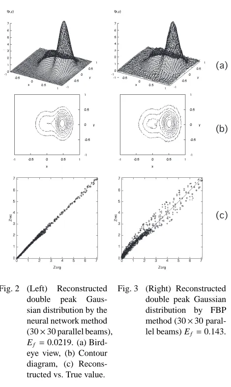
To demonstrate the two-dimensional image recon-struction by NNCM we prepare a set of line integrals for the double peak Gaussian distribution as a model of the numerical experiment. First we employed parallel-beam configuration with 30 directions with 30 parallel-beams each (30×30=900) and solved it by the NNCM system of Fig. 1. It should be noted that “NB”s in Fig. 1 represent neurons for the instrumental biases in CIT and are not used in the model data analysis of this section.
Though usually an activation function is not used in the output layer neurons, in our CT analysis method the following ”skimmer-type” activation function is used for stable convergence during the training process.
σ(x)=x+log(1+e−x), (6)
The functional error of the reconstructed image Ef is defined as
Ef =
N(zor−zrec)2
Mzmax ,
(7)
where zorg, zrec, zmax, and M denote the original, recon-structed images, the maximum value of the original image, and the total number of evaluation points, respectively.
The reconstructed image is shown in Fig. 2 with the result by the conventionally used filtered back projection (FBP) method in Fig. 3. The FBP method works very well if it is applied to a problem with a large amount of projec-tion data, but it gives a very poor result when it is applied to a problem with small amount of data as in this case. The errors of the reconstructed images by the NNCM and the FBP are Ef =0.0219 and Ef =0.143, respectively. It was also confirmed that the new method gave a rather good re-sult even for an extremely small amount of projection paths as 3×10=30 where Ef =0.034.
Fig. 2 (Left) Reconstructed double peak Gaus-sian distribution by the neural network method (30×30 parallel beams), Ef =0.0219. (a)
Bird-eye view, (b) Contour diagram, (c) Recons-tructed vs. True value.
Fig. 3 (Right) Reconstructed double peak Gaussian distribution by FBP method (30×30 paral-lel beams) Ef =0.143.
4. CT Image Reconstruction of
Iono-spheric Electron Density
Distribu-tion by NNCM
In this section, first, we describe some issues on the CT image reconstruction by NNCM specific to the iono-spheric electron density distribution, then numerical exper-iments for the data of the model ionosphere, and lastly the CT image reconstruction of the real observation data.
4.1
Some issues specific to the CT of the
ionospheric electron density distribution
We skip the technical details how to calculate the slant TEC values from the GPS observations. They are obtained from the group delays and the carrier phase advances of two radio signals from a GPS with different frequencies. The slant TEC Iij(t) at time t along the projection path be-tween the GPS j and the ground receiver i is the integrated value of the ionospheric and the plasmaspheric electron density which includes the instrumental biases of the trans-mitter in the satellite Bjand the ground receiver Bias
Iij(t)= rj
ri
N(r,t)d+Bi+Bj
(i=1, . . .I; j=1, . . .J),
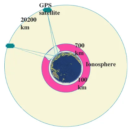
Fig. 4 Schematic diagram of the two-dimensional cross-section of the computational domain of CIT.
where N(r,t) is the electron density at the observation time t and the spatial position r, and I and J are the total
num-bers of the ground receivers and the GPS positions, re-spectively. The computational domain of the above inte-gral equations of N(r,t) is divided into two regions, i.e.,
the ionospheric region (lower region, 100 km∼700 km in altitude) and the plasmaspheric region (upper region, over 700 km in altitude), and the ionospheric region is our target for the CT image reconstruction (Fig. 4). The GPS orbits are located at 20,200 km in altitude.
When a sufficient number of the observation data for the slant TEC are available we can derive the ionospheric electron density N(r,t), and instrumental biases Biand Bj (“NB”) by solving the integral equation (Eq. (8)). The equation is descretized and the object function to be mini-mized is obtained as
E1=
i,j
U
u=1
αuN(ru,t)+Bi+Bj+P j i −I
j i(t)
2
,
(9) where u denotes the sampling point for the integration path within the ionosphere and Pijis the contribution of the plas-maspheric electron density to the slant TEC Iij(t).
As described previously the most significant issue in CIT by using the GPS signals is that high resolution in the vertical direction is difficult to attain because of scarcity of horizontal or near-horizontal projection paths. To cope with this problem and improve the vertical res-olution we use the information on the peak electron den-sity Nsiono(rionos ) ≡ NmF2 and the corresponding height
hmF2 obtained by the ionosonde measurement at the
s-th ionosonde observation station rionos . For this purpose we employed the following penalized object function as
E=E1+E2, (10)
E2= S
s=1
Ns(rionos )−N iono s (r
iono s )
2
, (11)
where S denotes the total number of the ionosonde sta-tions, “iono” denotes the measured value by the ionosonde, and is the penalty coefficient. In our analysis we used ionosonde data of only one station out of 4 ionosonde sta-tions.
Though it is not necessary to discretize the compu-tational domain as the mapping function realized by the multi-layer neural network is continuous, continuous treat-ment of the input space causes overfitting and makes the system unstable because of the finite number of the con-straints (number of projection paths). To avoid these de-fects, input space discretization is extremely effective. In the actual CIT, therefore, we discretize the temporal and spatial domain into finite-sized meshes. We set that the temporal resolution of the electron density distribution as
∆/2 = 7.5 min and we used the data observed during (t,t+∆). As for the spatial domain, the discretization is car-ried out so that more than one projection paths cross each three-dimensional mesh on average. For this reason we as-sume that the electron density is constant within an area of 0.5×0.5 deg (about 50 km×50 km) in latitude/longitude and 30 km in altitude.
To estimate the contribution of the plasmaspheric re-gion to the observed TEC value, we employ a simple diffusive equilibrium model proposed by Angerami and Thomas [22]. According to this model we assume the electron density distribution in the plasmasphere n(h) is decreasing exponentially from the top of the ionospheric region (h0 = 700 km) with the scale length Hs up to the satellite orbits (hsat =20200 km). Under this assumption the plasmaspheric contribution to the TEC value of the path (i,j), Pijis given as
Pij= 1
cosθ
hsat
h0
n(h0) exp
−h−h0
Hs
dh
≈ 1
cosθn(h0)Hs, (12)
where hsat is the altitude of each GPS andθis the incli-nation of the projection path with respect to the vertical direction.
4.2
Numerical experiment on the model data
calcu-lation, whereas the bias values of the satellites and ground receivers are assigned artificially. The values of NmF2 and
hmF2 at the actual ionosonde station located in Japan are
obtained from GCPM and used as the “observed” data. For the numerical experiment by NNCM we produced model observation data corresponding to the GCPM data of 1200-1215 JST, 22 December 2001 for 40 GEONET receivers located in Japan from Hokkaido to Okinawa. In both the model experiment and the real data analysis the observa-tion data from one ionosonde staobserva-tion located at Kokubunji (139.51 E, 35.74 N) among 4 ionosonde stations in Japan are employed and the data of 3 other ionosonde stations are used for validation. Total number of the projection paths P of 2128 is used and 20 sampling points for the integration are placed on each projection path. Taking into account of the errors of the preliminary calculations and the com-putational cost we decided to employ a 4-layered neural network with 3,12,12, 1 neurons in each layer. The cal-culations were carried out on a workstation with a Xenon 2.20 GHz CPU and it took about 10 min of CPU time to train the network (4000 iterations).
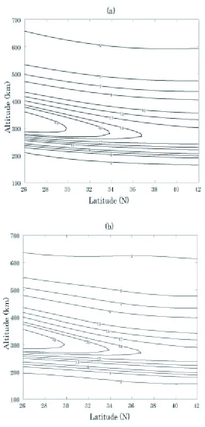
An example of the reconstructed density contour plot at the longitude of 137 E is shown in Fig. 5 b with the cor-responding true contour plot produced from the GCPM density distribution (Fig. 5 a). The average density error is 2.8×10¹⁶m−3in this calculation, which is very small in comparison with the typical peak density of 2×10¹⁸m−3. The bias values of the transmitters and the ground receivers were determined very accurately as 0.12 and 0.31 TECU (1 TECU=1×10¹⁶m−2).
4.3
Reconstruction of real electron density
distribution
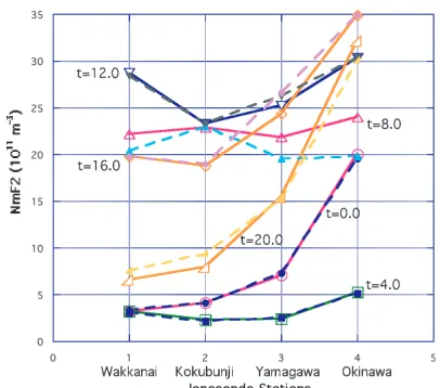
From the GPS data obtained by 40 different receivers over the Japanese archipelago and the ionosonde data ob-served at Kokubunji the actual three-dimensional iono-spheric electron density distribution of November 5, 2001 has been reconstructed. The observation data obtained within 15 min every hour are analysed to investigate the hourly variations of the ionospheric electron density dis-tribution from 0000 to 2400 JST. To confirm that the suf-ficiently high vertical resolution is attained by NNCM the peak density values NmF2 and the peak density heights
hmF2 at the ionosonde stations, Wakkanai, Yamagawa,
and Okinawa in addition to Kokubunji whose data were used for training are plotted over 24 hr on Novemver 5, 2001 and compared with the observed data (Figs. 6 and 7). Agreement between the reconstructed values and the ob-served values are very good (the root mean square error of the peak density at the ionosonde sites is∼7 %), from which it can be concluded that the reconstructed density distribution agrees with the true density distribution even at points apart from the ionosonde station used for train-ing.
Fig. 5 Contour plot of the model (a) and reconstructed (b) den-sity distributions at longitude 137 E. The unit of denden-sity is 1011m−3.
5. Conclusion
Fig. 6 Comparison of the ionosonde observed NmF2 (solid line) and the corresponding values reconstructed by NNCM (broken line) at time t=0, 4, 8 12, 16, 20.
Fig. 7 Comparison of the ionosonde-observed hmF2 (solid line) and the corresponding values obtained by NNCM (bro-ken line). The unit of hmF2 is the kilometer.
network is a function approximation with variable basis function though usually CIT is carried out based on the “fixed” orthogonal basis functions or EOF. Comparison of our results on the real observation data with those by other methods is rather difficult because observation datasets are not the same, i.e., conditions of the ionosphere, positions of the satellites and the ground receivers are all different and, moreover, detailed quantitative data are not published usually, but our result is presumed among best values ob-tained by other three dimensional CITs from the viewpoint of the reconstruction errors of the NmF2 data [13, 14], and the results of the model data analysis show that the error is limited almost by the spatial grid size.
NNRMT is applicable to wide range of problems other than the tomographic image reconstruction described in this paper [25–30]. In this method various excellent fea-tures of the neural network are utilized and even numerical
formulation of rather complicated problem can be carried out comparatively easily.
[1] T. Takeda, A. Liaqat and M. Fukuhara, Proc. Internat. Workshop on Modern Sci. and Technol. 2002 (Sept. 19-20, Univ. of Electro-Commun., Tokyo, 2002) p.145.
[2] X.F. Ma, M. Fukuhara and T. Takeda, Nucl. Instrum. Meth-ods in Phys. Res. A 449, 366 (2000).
[3] X.F. Ma, T. Maruyama, G. Ma and T. Takeda, J. Geophys. Res. 110, A05308, doi:10.1029/2004JA010797 (2005). [4] J.R. Austen, S.J. Franke and C.H. Liu, Radio Sci. 23, 299
(1988).
[5] T.D. Raymund et al., Radio Sci. 25, 771 (1990).
[6] F.J. Fremouw, J.A. Secan and B.M. Howe, Radio Sci. 27, 721 (1992).
[7] M. Kunitake et al., Ann. Geophysicae 13, 1303 (1995). [8] G.A. Hajj and L.J. Romans, Radio Sci. 33, 175 (1998). [9] L.-C.Tsai et al., Earth Planets Space 53, 193 (2001). [10] M. Garcia-Fernandez, M. Hernandez-Pajares, M. Juan and
J. Sanz, J. Geophys. Res. 108(A9), 1338, doi:10.1029/ 2003JA009952 (2003).
[11] A.J. Hansen, T. Walter and P. Enge, Ionospheric correction using tomography, Proceedings of the Institute of Naviga-tion GPS’97, 249 (1997).
[12] M.J. Hernandez-Pajares, M. Juan and J. Sanz, J. Geophys. Res. 103, 20,789 (1998).
[13] S. Schl¨uter, C. Stolle, N. Jakowski and C. Jacobi, “Mon-itoring the 3 Dimensional Ionospheric Electron Distribu-tion based on GPS Measurements” in First CHAMP Mis-sion Results for Gravity, Magnetic and Atomspheric Stud-ies (Springer Verlag, Berlin, 2003).
[14] M. Garcia-Fernandez, A. Saito, J.M. Juan and T. Tsuda, J. Geophys. Res. 110, A11304, doi:10.1029/2005JA011037 (2005).
[15] S. Miyazaki et al., Bull. Geogr. Surv. Inst. 43, 23 (1997). [16] S. Haykin, Neural Networks: A Comprehensive foundation,
2ndEd. (Prentice Hall, Upper Saddle River, NJ, 1999). [17] R. Rojas, Neural Networks: A Systematic Introduction
(Springer, Berlin, 1996).
[18] D.E. Rumelhart, G.E. Hinton and R.J. Williams, Nature 323, 533 (1986).
[19] K. Funahashi, Neural Networks 2, 183 (1989). [20] H. White, Neural Networks 3, 535 (1990). [21] T. Poggio and G. Girosi, Science 247, 978 (1990). [22] J.J. Angerami and J.O. Thomas, J. Geophys. Res. 69, 4537
(1964).
[23] D.L. Gallagher and P.D. Craven, J. Geophys. Res. 105, 18, 189 (2000).
[24] D. Blitza, International Reference Ionosphere 1990, NSSDC 90-22, Natl. Space Sci. Data Center, Greenbelt, Md (1990).
[25] X.F. Ma and T. Takeda, Nucl. Instr. Methods in Phys. Res. A 492, 178 (2002).
[26] A. Liaqat, M. Fukuhara and T. Takeda, Comput. Phys. Commun. 141, 350 (2001).
[27] A. Liaqat, M. Fukuhara and T. Takeda, Comput. Phys. Commun. 150, 215 (2003).
[28] A. Liaqat, M. Fukuhara and T. Takeda, Month. Weather Rev. 131(8), 1696 (2003).
[29] J. Wu, M. Fukuhara and T. Takeda, Ecological Modeling 189, 289 (2005).