Advanced High-order Hidden Bivariate Markov Model Based Spectrum Prediction

Advanced High-order Hidden Bivariate Markov

Model Based Spectrum Prediction

Zhiming

Hong

,

Yanxiao

Zhao

,

Yu

Luo

,

Guodong

Wang

and

Lina

Pu

South Dakota School of Mines and Technology, Rapid City, SD 57701 USA.

Abstract

The majority of existing spectrum prediction models in Cognitive Radio Networks (CRNs) don’t fully explore the hidden correlation among adjacent observations. In this paper, we first develop a novel prediction approach termed high-order hidden bivariate Markov model (H2_{BMM) for a stationary CRN. The proposed} H2_{BMM leverages the advantages of both HBMM and high-order, which applies two dimensional parameters,} i.e., hidden process and underlying process, to more accurately describe the channel behavior. In addition, the current channel state is predicted by observing multiple previous states. Afterwards, the mobility of secondary users is fully considered and we propose an advanced approach based on H2BMM, termed Advanced H2BMM, to accommodate a mobile CRN. Extensive simulations are conducted and results verify that the prediction accuracy is significantly improved using the proposed (H2BMM. The Advanced H2BMM is also evaluated with comparison to H2BMM and results show considerable improvements of H2BMM in a mobile environment.

Receivedon 7 December 2017;acceptedon 9 December 2017;publishedon 12 December 2017

Keywords: cognitive radio network, spectrum prediction, high-order hidden bivariate Markov model.

Copyright © 2017 Zhiming Hong et al., licensedto EAI. Thisis anopen access article distributedunder theterms of theCreativeCommonsAttributionlicense(http://creativecommons.org/licenses/by/3.0/),whichpermitsunlimited use,distributionandreproductioninanymediumsolongastheoriginalworkisproperlycited.

doi:10.4108/eai.12-12-2017.153466

1. Introduction

Cognitive Radio Networks (CRNs) are commonly per-ceived as a promising solution to the issue of spectrum scarcity. In CRNs, Primary Users (PUs) and Secondary Users (SUs) refer to the authorized and unauthorized users of allocated channels, respectively [1]. SUs are allowed to access channels opportunistically without harmful interferences to PUs [2]. To implement CRNs successfully, spectrum sensing is an essential process, in which SUs must obtain awareness about the spectrum usage to avoid destructive interferences to PUs [3].

A traditional CRN requires SUs to continually conduct a spectrum sensing process [4]. Specifically, time is divided into slots which consist of a small portion of sensing period, followed by a relative long period for data transmission. SUs conduct regular sensing and update the sensing result every time slot, which leads to high computational complexity [5]. To speed up the sensing process and save more time for transmission, spectrum prediction is a favorable

∗_{Corresponding author. Email:[email protected]}

technology. Spectrum prediction refers to the process of estimating the future channel occupancy status by analyzing sensing history [6]. With prediction, SUs are not required to sense the channel every time slot and hence the time for data transmission is prolonged.

A few spectrum prediction schemes have been proposed in the recent literature. Authors in [7] summarize several state-of-the-art spectrum prediction techniques and illustrate their applications. In [8] [9] [10], Markov related prediction algorithm has been improved from Hidden Markov Model (HMM) to high-order HMM and Hidden Bivariate Markov Model (HBMM). The standard HMM [8], also named the first-order HMM, solely depends on one immediately prior state and the correlation with other previous states is not fully explored. To improve the accuracy, a high-order HMM is proposed and evaluated in [9] where the current channel state depends on more than one prior states. In addition, studies discover that the geometric distribution characteristic of HMM is not suitable for describing channel behaviors, especially when bursty transmissions occur [11]. To better model the cognitive radio channel, hidden bivariate Markov model (HBMM)

is proposed and applied to spectrum prediction in [10]. The main idea of HBMM is to further divide a channel state into multiple sub-states, forming an underlying process, so that the channel sub-state dwell time follows a Phase distribution.

As mentioned above, HBMM and high-order HMM are proposed separately to improve the standard HMM from two perspectives. In our paper, we first consider a stationary CRN and propose a novel prediction approaches, termed High-order Hidden Bivariate Markov model (H2BMM), by leveraging the advantages of both high-order and HBMM. H2BMM is to apply two dimensional parameters, i.e., hidden process and underlying process, to more accurately describe the channel behavior. In a stationary CRN, individual stationary SUs conduct H2BMM to complete the tasks of sensing and prediction. Afterwards, we extend H2BMM to a mobile CRN since mobility is an inherent feature in a wireless environment. In a mobile CRN, when SUs move, it is difficult for an individual SU to analyze the activity patterns of PUs along with its moving path [12]. Therefore, the concept of cooperative sensing [13] is adopted and a base station will collect sensing information from mobile SUs to analyze and predict channel states. Besides, it is challenging to continuously sense PUs’ status due to the mobility of SUs. To accommodate a mobile CRN, we improve H2BMM, termed Advanced H2BMM, by considering the discontinuous sensing behaviors of mobile SUs, .

Our main contributions are briefly summarized as below:

• For a stationary CRN, a novel High-order Hidden Bivariate Markov Model (H2_{BMM) based}

spectrum prediction approach is proposed to fully inherit the strengths of high-order HMM and HBMM. In this approach, the prediction accuracy is enhanced by considering a underlying process and observing multiple previous states as well.

• Theoretical analysis is tailored to the training and prediction process for H2BMM. The dimensional-ity of transition probabildimensional-ity matrix in a standard HBMM is two. In H2_{BMM, we increase the}

dimen-sionality so that one state depends on previous

m(m≥2) states. Accordingly, analysis of forward and backward possibilities is revised to calculate the conditional probability of the current state under its previousmand futuremstates.

• For a mobile CRN, we further improve the training algorithm of H2BMM to adapt to the discontinuous sensing behaviors of mobile SUs because H2BMM is originally developed when both PUs and SUs are fixed. The new training method of Advanced H2_{BMM can}

achieve remarkably higher prediction accuracy in a mobile environment.

The rest of the paper is organized as follows. Related work on spectrum prediction is introduced in Section 2. Section 3 presents the detailed description of the proposed H2BMM based spectrum prediction approach, along with theoretical analysis. Section

4 introduce the Advanced H2BMM for a mobile environment. Simulation results are described in Section5and conclusions are drawn in Section6.

2. Related Work

The growing concern over the spectrum scarcity has inspired considerable research on spectrum prediction in CRNs. Spectrum prediction is a necessary mean to address the spectrum fluctuation problem. Several com-mon spectrum prediction algorithms, including HMM, HBMM and high-order HMM, are first introduced in this section, followed by a comparison among these solutions.

2.1. Hidden Markov Model (HMM) Based Prediction

In CRNs, the two-state channel model is commonly used, in which “0” and “1” indicate the channel being idleandbusy, respectively. Since the actual channel state is typically hidden from SUs in HMM [8] [14], letX=

{“0”, “1”} denotes the actual and hidden state space, while Y ={“0”, “1”} denote the observation/sensing state space.

The model training process is to adjust each element value of state transition probability matrix

A= [aij], i, j∈X and emission probability matrix B=

[bij], i, j∈Y [15]. As shown in Fig. 1, each element

aij of state transition probability matrix A denotes

the probability that the hidden channel state transfers from state “i” to state “j”, while each element bij

of emission probability matrix denotes the probability that hidden channel state “i” is observed as state “j” [16]. With the trained matrices and observation history, we are able to calculate the mostly likely hidden states chain and future states. In [17], HMM is applied to diagnose electronic circuit fault using high-order spectral analysis, but the high-order concept is different from that in our paper.

2.2. Hidden Bivariate Markov Model

HBMM can be viewed as an extension of standard HMM [18]. The main advantage of HBMM [10] [14] is that the dwell time in a given state has a discrete phase-type distribution which is more suitable for modeling a cognitive radio channel than the geometric dwell time distribution of HMM. In HBMM, each channel state contains r sub-states denoted by {Sn}. Let {Zn=

ܺ

ൌ Ͳ

ܺ

ൌ ͳ

ܻ

ൌ Ͳ

ܻ

ൌ ͳ

ܽͲͲ

ܽͲͳ

ܽͳͳ

ܽͳͲ

ܾͲͲ ܾ_Ͳͳ ܾ_ͳͲ ܾͳͳ

Figure 1. Hidden Markov Model (HMM) [14]

Markov chain. {Xn} is referred to as the state process,

while {Sn} is the underlying process. The observable

process denoted by {Yn} is obtained by observing the

state process {Xn} through a Gaussian memoryless

channel. The transition matrix can be expressed by:

G=

[

G11 G12

G21 G22

]

, (1)

whereGab ={gab(ij), i, j= 1,2, . . . , r}is anr×rmatrix.

2.3. High-order HMM

In the conventional first-order HMM, the prediction of current state is solely determined by its immediate previous state. High-order HMM [9] [14], instead, make predictions by considering multiple previous states [19]. As a result, first-order HMM and high-order HMM possess different transition matrix. Taking 2nd-order HMM [20] as an example, the size of transition matrixG

isn×n×nand each elementgijkmeans the probability

that the hidden channel state transfers from state “i” to state “j” and then to state “k”. In general, when the order of high-order HMM increases, the performance is much better than the traditional HMM [21].

In summary, these typical prediction techniques have their advantages and disadvantages. There are two key problems of HMM. One is that the geometric dwell time distribution characteristic of the HMM is not adequate for modeling a cognitive radio channel, especially when bursty transmissions happen. Another one is that HMM is not able to fully explore the hidden correlation among adjacent observations because a state only depends on its previous one state. HBMM can be viewed as a modified HMM with better dwell time distribution characteristic through extending each hidden state to several sub-states. High-order HMM solves the limitation of low correlations and can obtain a better

performance. Therefore, we combine the concept of High-order HMM and HBMM, and then propose a H2BMM based spectrum prediction approach.

3. H

BMM Based Spectrum Prediction

In this section, the proposed H2BMM based spectrum prediction will be introduced. Before we delve into the details, the scenario of prediction on spectrum sensing is described first. We assume that the channel state alternates between “0 (idle)” and “1 (busy)”. An SU observes the received signal and makes a sensing decision for the channel state: either “0 (idle)” or “1 (busy)”. Taking energy detection as an instance, if the received energy amplitude exceeds a predefined threshold, the channel is perceivedbusy, otherwise the channel is determined asidle.

3.1. H

BMM Parameters

Due to signal noise and interference, the sensed channel state does not necessarily represent the actual state. Therefore, we can view that the actual channel state is hidden from the SU. Let X={“0”, “1”} denotes the hidden state space, with “0” and “1” indicating that the channel is idle and busy, respectively. Similarly, let

Y ={“0”, “1”}denote the observation state space, with “0” and “1” indicating that the spectrum sensing results is idle and busy respectively. The principle of spectrum prediction is to predict future channel states from the historical channel states.

In terms of notation, capital letters are used to denote random variables and lower case letters to denote their realizations. Let{Xn},{Yn}and{Sn}represent the hidden

process (i.e., the actual channel states), observation process (i.e., sensing results of channel state) and underlying process. Note that the underlying process

{Sn}takes values inS={1,2, . . . ,5}, which implies that

each channel state inX,idle(“0”) orbusy(“1”), contains 5 sub-states. The role of the underlying process{Sn}is

to facilitate mathematical analysis, i.e., induce a phase-type distribution on the dwell times of{Xn}in theidle

orbusystate. Let{Zn= (Xn, Sn), n= 0,1, . . . , N}denotes

the discrete-time bivariate Markov chain.

We assume that energy detection is employed for spectrum sensing and when channel state is idle, the observed signal strength {Yn} follows a Gaussian

distribution with µ0 mean and σ02 variance. Similarly,

when channel state is busy, {Yn} follows a Gaussian

distribution withµ1mean andσ12variance.

The H2BMM parameters, denoted byϕ= (π, G, µ, R), consist of an initial probability distribution π, a transition matrix G, a vector of mean observed signal strengths µ={µ0, µ1}, and a vector of observed signal

example, the size of G is n×n×n for 2nd-order H2BMM and each element gijk means the probability

that the channel state transfers from state “i” to state “j” and then to state “k”.

To better understand the concept of H2BMM, we illustrate the 2nd-order H2BMM with two sub-states in Fig.2. As can be seen, each main state contains two sub-states and state transitions occur among these total four sub-states. Since this is for the 2nd-order model, the current state is related to its previous two states, i.e., from slotn−2 ton−1 and then ton.

Idle Xn-2= 0

Sn-2= 0

Idle Xn-2= 0

Sn-2= 1

Busy Xn-2= 1

Sn-2= 0

Busy Xn-2= 1

Sn-2= 1 Slot n-2

Idle Xn= 0

Sn= 0

Idle Xn= 0

Sn= 1

Busy Xn= 1

Sn= 0

Busy Xn= 1

Sn= 1 Slot n

Idle Xn-1= 0

Sn-1= 0

Idle Xn-1= 0

Sn-1= 1

Busy Xn-1= 1

Sn-1= 0

Busy Xn-1= 1

Sn-1= 1 Slot n-1

Figure 2. HHBMM Concept

3.2. H

BMM

In this subsection, the proposed H2BMM prediction procedures will be described in detail. Specifically, three major steps are involved. The first step is to generate a hidden channel state chain and observation chain as well. Then a training process is required for H2_{BMM, in which the widely used Baum-Welch}

algorithm [22] is adopted. Last, the strategy of making a prediction decision is introduced. The following will detail each main step.

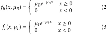
1) Generating hidden state chain and observation chain For the channel states, we include the duration time for each state. It is assumed that the duration/dwell time of channel busy and idle states follows an exponential distribution, which is a special case of Phase distribution. That is, we consider the channel activity as a two-state model which incorporates busy andidledurations. The exponential distribution is used to generate a predictable hidden state chain {Xn, n=

0,1, . . . ,2N},

fB(x, µB) =

{

µBe−µBx x≥0

0 x <0 (2)

fI(x, µI) =

{

µIe−µIx x≥0

0 x <0 (3)

whereµBandµI arebusyandidleduration parameters.

The channel duration distribution functions deter-mine how long (i.e., how many time slots) the chan-nel will remain in the current state. It is known the dwell/duration time of a channel state can be any positive value. Here we are interested in the channel state remaining for one time slot. Therefore, a new term is introduced calledtransient state probabilityto indicate the probability of channel state (idleorbusy) remaining for only one time slot. The transient state probability significantly affects the performance of spectrum pre-diction, which will be evaluated in Section 5. We use transient state probabilityPB→I to represent the

proba-bility of channel staying onbusyfor only one time slot. Similarly,PI→Bindicates the probability ofidlestate for

one time slot. For example, in the case of PB→I = 0.5

and PI→B= 0.8, the possibility of one-slot dwell time

in busy state is 50%, and the probability of one-slot dwell time inidlestate is 80%. In other words, observing three consecutive time slots, if the current slot isbusy, previous and next slots are bothidle, this (i.e., staying in busyfor only one time slot) occurs with a probability of 50%. If the current slot isidle, previous slot isbusyand the next slot changes tobusy, the likelihood of this (i.e., staying inidlefor only one time slot) happening is 80%.

瀋 濃 濃濁濄 濃濁濅 濃濁濆 濃濁濇 濃濁濈 濃濁濉 濃濁濊

濹澻瀋澿煱澼 濄 濃濁濌濃濇濋濆濊 濃濁濋濄濋濊濆濄 濃濁濊濇濃濋濄濋 濃濁濉濊濃濆濅 濃濁濉濃濉濈濆濄 濃濁濈濇濋濋濄濅 濃濁濇濌濉濈濋濈

0 1 2 3 4

Ex

pone

nti

al

Dist

ribut

ion

Time Slots

Figure 3. Illustration of calculating the transient state probability from an exponential duration distribution of a channel state

Fig. 3 illustrates an exponential duration/dwell distribution of a channel state. Since the transient state probability is defined as the probability of staying on the current state for one time slot, it is actually the integral of channel duration distribution functions from 0 to 1 (time slot), i.e., the shaded area in Fig.3.

As a result, the formulas of PB→I and PI→B can be

derived as below:

PB→I =

∫1

0

fB(x, µB)dx (4)

PI→B=

∫₁

0

In addition, a signal strength observation chain

{Yn, n= 0,1, . . . ,2N}is generated by applying Gaussian

distribution. As mentioned previously, {Yn} follows a

Gaussian distributionN(µ0, σ02) when{Xn}is idle, and {Yn} follows a Gaussian distribution N(µ1, σ12) when {Xn}is active.

2. H2BMM Training

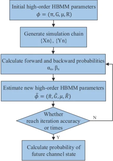
After generating the training sequence, H2BMM is trained using the generated sequence. The widely used training algorithm of HMM is Baum-Welch algorithm. Based on the Baum-Welch algorithm, we design the training and prediction algorithm for H2_{BMM. The}

m order HBMM training flow is summarized in Fig. 4. Once a new piece is received, the oldest piece will be abandoned. Given an initial parameter estimateϕ= (π, G, µ, R) and a piece of signal strength observations {Yn, n= 0,1, . . . , N}, a parameter estimate

ˆ

ϕ= ( ˆπ,G,ˆ µ,ˆ Rˆ) with a higher likelihood is computed. Forward and backward probabilities are critical to estimate the parameter ϕ= (π, G, µ, R), which will be factored in Eq.9. After a certain number of iterations, a more accurate parameter estimate will be obtained.

Initial high-order HBMM parameters

= (!, G,", R)

Generate simulation chain {Xn}, {Yn}

Calculate forward and backward probabilities

α_n,βn

Estimate new high-order HBMM parameters

!_{= ("#,$!,%,&!)}

Whether reach iteration accuracy

or times

Calculate probability of future channel state

Y

N

Figure 4. High-Order HBMM (H2BMM) training flow

• Forward Probability

We define a forward probability, αkr(n), k∈X, r∈

S, as the probability of current state Zn ={Xn, Sn}

being (k, r) under the condition of previous n vectors

{y0, . . . , yn−1}. Define a 10×10 block diagonal matrixBn,

with its diagonal blocks given by{p(yn|Xn=k)I, k∈X}.

I is a 5×5 identity matrix. In Eq. 6, α(n) denotes a 1×10 vector of{α01(n), . . . , α05(n), α11(n), . . . , α15(n)}.

α(0) =πB0;

. . .

α(m−1) =α(m−2)GBm−1;

. . .

α(n) =

[(_m ∏

i=1

α(n−i)

)

G

]

Bn, n=m, . . . , N .

(6)

whereπdenotes the initial states probability distribu-tion and m denotes the order of H2BMM. The recur-sive calculation of forward probability uses previous

mforward probability. Therefore, we first calculate the forward probability of first m states: α(0) to α(m−

1), from which α(m) can be determined. By repeating the process, with the forward probability of previous

m states, forward probability of the following state,

α(n), n=m+ 1, . . . , N, can be obtained.

• Backward Probability

Similarly, we define a backward probability,

βkr(n), k∈X, r ∈S as the probability of current

state Zn being (k, r) under the vectors of

{yn+1, . . . , yN}. In Eq.7,β(n) denotes a 1×10 vector of

{β01(n), . . . , β05(n), β11(n), . . . , β15(n)}.

β(N) =1′

. . .

β(N −m+ 1) =β(N−m+ 2)BN−m+2G′;

. . .

β(n) =

[( ₁ ∏

i=m

β(n+i)

)

Bn+1

]

G′,

n=N−m, . . . ,0.

(7)

where “′” denotes matrix transpose and “1” denotes a column vector of all ones. We calculate the backward probability of last m states:β(N) toβ(N−m+1). With the backward probability of last m states, backward probability of the previous one state, β(n), can be determined.

• Parameter Estimation

Applying the forward probability and backward probability formulas above, we can calculate the condi-tional probability p(zn−m, ..., zn−1, zn|y0N;ϕ), n= 2, . . . , N

for H2BMM in Eq.8.

p(zn−m, ..., zn−1, zn|y0N;ϕ) =

G(zn−m, ..., zn−1, zn)Q(n)

∑

zn−m,...,zn−1,zn

G(zn−m, ..., zn−1, zn)Q(n)

,

whereQ(n) =α(n−2)β(n)p(yn|xn).

The left side of this formula means the probability of m+ 1 states, zn−m, ..., zn−1, zn, appearing in the

whole observation sequence {Yn}. The whole training

computation complexity rises exponentially along with the increase of order index m, which leads to high computation delay. Taking both performance and complexity into consideration, we choose the order index to be two. In 2nd-order H2BMM, current channel state depends on previous two states. Then we can regenerate the transition matrixG:

ˆ

gabc(ijk) =

N

∑

n=2

p(zn−2= (a, i), zn−1= (b, j), zn= (c, k)|y0N;ϕ)

∑

(c,k)∈Z N

∑

n=2

p(zn−2= (a, i), zn−1= (b, j), zn= (c, k)|y0N;ϕ)

(9)

where ˆgabc(ijk) indicates the possibility of transferring

fromzn−2= (a, i) tozn−1= (b, j) and then tozn= (c, k).

In a standard HBMM, one state only depends on its previous one state. Each element of transition matrix of HBMM, G(Zn−1, Zn), means the possibility

of transferring from Zn−1 to Zn. In our proposed

H2BMM, one state depends on previous two states. We redesign the training algorithm to generate a transition matrix with 3 dimensionalities. Each element of this 3D transition matrix, G(Zn−2, Zn−1, Zn), means

the possibility of transferring from Zn−2, Zn−1 to Zn.

The same as HMM, mean signal strengths vector

µ and signal strengths variances vector R are also updated in each iteration. The variation of interferences throughout the simulation can reflect on µ and R

because prediction model should be updated during the whole simulation period not just the initial training process.

3. Prediction Decision

Given the observation chain {Yt}, a most likely {Zt}

can be calculated. If the last two states of{Zt}arezn−1

and zn, then the possibility of next state being zn+1 is

G(zn−1, zn, zn+1). Any possiblezn+1has its corresponding

possibility. As we know, in a 2D matrix, if we specify the first one dimensionality, a vector can be selected. Similarly, in a 3D matrix, if we specify the first two dimensionalities, a vector can also be selected. Then the next state probability distribution can be expressed by

P(Zn+1) =G(Zn−1, Zn,:) (10)

where “:” denotes any possiblezn. Therefore,P(Zn+1) is

a vector where each element indicates the probability of a possiblezn+1.

Since channel state is eitheridleorbusyand each state has 5 sub-states, P(Zn+1) is a vector with length of 10.

The first 5 elements ofP(Zn+1) mean the 5 sub-states of

idleand the last 5 elements ofP(Zn+1) mean the 5

sub-states ofbusy. To determine the most possiblezn+1, we

should find the maximum value ofP(Zn+1). If the order

number of the maximum element in P(Zn+1) iss, the

next channel stateXn+1is

Xn+1=

{

0 s≤5

1 s >5 (11)

If the maximum value ofP(Zn+1) is located inside the

first 5 elements, next one channel stateXn+1 should be

idle, otherwiseXn+1should bebusy.

Multi-step prediction can be conducted the same as 1-step prediction. After we predict the next one channel state{Xn+1}, the previousn+ 1 channel states

are viewed as historical data. Then the next two channel

{Xn+2}can be predicted.

4. Advanced H

BMM Based Spectrum Prediction

As presented in Section3.2, the H2BMM is designed for stationary SUs to conduct spectrum prediction. In this section, a mobile CRN is considered and an extension of H2BMM, named Advanced H2BMM, is proposed.

4.1. Scenario

In a mobile CRN, SUs sense channel statuses and report sensing results to a Control Base Station (CBS) during their movement. The CBS is responsible for predicting the channel status. When an SU is moving towards a PU, at first, PU is out of the sensible range of SU, i.e., SUs can not sense the PU’s existence. Hence, SUs determine that channel is in theidlestate in this situation. After entering the sensible region of PU, SUs are able to sense the channel status.

The Advanced H2BMM is applied to analyze historical sensing information and then predict future channel status. If the next channel state is predicted to be busy, SUs should exit the current channel in advance. After the channel is predicted to remainidlestate, SUs can remain communications.

4.2. Advanced Training Algorithm

pieces of sensing data. In order to keep prediction matrix adapted to latest spectrum environment, we set T Htpn as the threshold of training piece number.

Therefore, instead of a whole sensing sequence{Yn}, a

CBS is likely to receive many sensing pieces as shown in Eq.12.

piece1 :Yn1={y1, y2, . . . , yi}

piece2 :Yn2={y1, y2, . . . , yj}

. . .

piece m:Ynm={y1, y2, . . . , yk}

(12)

where Ynm indicates mth sensing piece received by

CBS. The length of received sensing pieces is random and there is no relationship between piece number and piece length. Piece length is random and could be any integer from 1 to simulation length. The training algorithm of the Advanced H2BMM is revised by utilizing pieces of sensing sequences to update the training matrix, based on Subsection 3.2. The improvements are described as below.

• Forward Probability

In the Advanced H2BMM, the forward possibility is calculated for each piece of sensing, which is denoted byα(n)piece i. Then the forward recursion is updated as

below, based on Eq.6in subsection3.2:

α(0)piece i=πB0;

. . .

α(m−1)piece i=α(m−2)piece iGBm−1;

. . .

α(n)piece i=

[(_m ∏

i=1

α(n−i)piece i

)

G

]

Bn, n=m, . . . , N .

(13)

• Backward Probability

Similarly, the backward possibility for each piece of sensing, denoted by the β(n)piece i, is derived based on

Eq.7in subsection3.2, as follows:

β(N)piece i=1′

. . .

β(N −m+ 1)piece i=β(N −m+ 2)piece iBN−m+2G′;

. . .

β(n)piece i=

[( ₁ ∏

i=m

β(n+i)piece i

)

Bn+1

]

G′,

n=N −m, . . . ,0.

(14)

• Parameter Estimation

So far we have calculated the forward and backward possibilities for each sensing piece. By considering all pieces, the conditional probability is calculated in Eq.

15, which is revised based on Eq.8in subsection3.2.

p(zn−m, ..., zn−_∑1, zn|y0N;ϕ) = all pieces

G(zn−m, ..., zn−1, zn)Q(n)

∑

all pieces

∑

zn−m,...,zn−1,zn

G(zn−m, ..., zn−1, zn)Q(n)

,

(15)

5. Simulation Results

In this section, the performance of H2BMM and Advanced H2BMM are evaluated. First, H2BMM is compared with two traditional models in a stationary CRN environment. For a mobile CRN environment, the Advanced H2BMM is compared with H2BMM to verify its advantages.

5.1. H

BMM in Stationary CRNs

The proposed H2_{BMM is evaluated in comparison with}

HMM and HBMM under a stationary environment, where both PUs and SUs are fixed. There are three key factors which affect the spectrum prediction performance of H2BMM, i.e., transient state probability, prediction steps and order of H2BMM. We evaluate the corresponding impact on the prediction performance by adjusting these factors.

First, prediction accuracies affected by the transient state probability are evaluated. As presented in Section

3, transient state probability PB→I and PI→B are

calculated in Eqs. (4) and (5). The values ofPB→I and

PI→B can be altered by adjusting parameters of µB

and µI, to simulate a various spectrum environment.

Specifically,PB→I is fixed to 0.8 whilePI→Bis increased

from 0.1 to 0.9, correspondingly µB is fixed to 1.61

whileµI is increased from 0.11 to 2.30. We compare the

prediction accuracy of H2_{BMM, HBMM and HMM with}

1-step prediction. Results are shown in Fig.5.

Comparing these three lines in Fig 5, they have a similar V-shaped trend but H2_{BMM obtains higher}

prediction accuracy than HMM and HBMM. From the line of 1-step HBMM in Fig. 5, it can be seen that the prediction accuracy is a V-shaped graph, starting considerably high around 87% when PI→B= 0.1, then

it gradually decreases whilePI→B increases from 0.1 to

0.5. WhenPI→B= 0.5, the prediction accuracy reaches

the lowest point. Afterwards, it continuously increases when PI→B increases from 0.5 to 1. This trend is

reasonable and can be interpreted as follows. When

PI→B= 0.1, it means the probability of channel state

0.1 0.2 0.3 0.4 0.5 0.6 0.7 0.8 0.9 Transient State Probability P

I→B 65%

70% 75% 80% 85% 90% 95% 100%

Prediction Accuracy

1-step H2BMM (2nd-order) 1-step HBMM 1-step HMM

Figure 5. Prediction accuracy of H2BMM, HBMM and HMM

whenPB→I = 0.8,PI→B from 0.1 to 0.9

The prediction accuracy is lowest when the value of

PI→B is equal to 0.5. This is due to the fact when

the transient state probability is close to 0.5, the possibility is approaching 50% for the next state to be idleorbusy, which results in random and unpredictable spectrum pattern. Similarly, the spectrum pattern becomes stronger whenPI→B increases from 0.5 to 0.9.

Consequently, the prediction accuracy keeps rising and achieves the highest point again whenPI→B= 0.9.

0.1 0.2 0.3 0.4 0.5 0.6 0.7 0.8 0.9

Transient State Probability P

I→B

30% 40% 50% 60% 70% 80% 90% 100%

Prediction Accuracy

P_{B → I}=0.8 1-step H2_{BMM (2nd-order)} P_{B → I}=0.8 3-step H2_{BMM (2nd-order)} P_{B → I}=0.8 5-step H2_{BMM (2nd-order)}

P_{B → I}=0.5 1-step H2_{BMM (2nd-order)} P_{B → I}=0.5 3-step H2_{BMM (2nd-order)} P_{B → I}=0.5 5-step H2_{BMM (2nd-order)}

Figure 6. Prediction accuracy of H2BMM (2nd-order) when

PB→I is0.8and0.5

Second, the performance of 2nd-order H2BMM is evaluated when PB→I is set to 0.8 and 0.5,

correspondinglyµB is set to 1.61 and 0.69 respectively,

while PI→B increases from 0.1 to 0.9. The prediction

accuracy of 1-step, 3-step and 5-step prediction are calculated, respectively. k-step prediction refers to that

the channel states of next k slots instead of only one slot are predicted for each prediction. Results for 2nd-order H2BMM are depicted in Fig6.

In contrast, when the value ofPB→I is set to 0.5 and

other factors are kept unchanged, all the prediction accuracies obtained by these three algorithms are relatively lower. Especially when the transient state probability reaches 0.5, the spectrum pattern becomes more and more random which greatly reduces the predict accuracy. However, the 1 step H2BMM still achieves reasonable prediction accuracy even when the transient state probability reaches 0.5. In addition, the effect of prediction steps can also be observed from Fig.6. The prediction of the 1-step achieves the highest accuracy, and the prediction accuracy decreases with the increase of steps.

0.1 0.2 0.3 0.4 0.5 0.6 0.7 0.8 0.9

7UDQVLHQW6WDWH3UREDELOLW\ P

I→B

0% 5% 10% 15% 20% 25% 30%

False Alarm Probability

1-step H2_{BMM (2nd-order)}

3-step H2_{BMM (2nd-order)}

5-step H2BMM (2nd-order) 1-step HBMM

3-step HBMM 5-step HBMM

Figure 7. False alarm possibility of HBMM (1st-order) and

H2BMM (2nd-order)

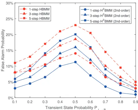
Third, the false alarm and miss detection of the prediction achieved by the H2BMM are evaluated. The false alarm probability means that the channel state is falsely detected as busy when the channel is actuallyidle, while miss detection is the opposite, that is, the channel state is false perceived as idle when the channel is actually busy [23]. In addition, order of H2BMM indicates the correlation degree among adjacent observations. Higher order means the model can better explore the hidden correlation information from training sequences. In this simulation, we mainly compare the false alarm and miss detection achieved by the 1st-order H2BMM, which becomes HBMM, and 2nd-order H2BMM.

0.1 0.2 0.3 0.4 0.5 0.6 0.7 0.8 0.9 Transient State Probability P

I→B

0% 5% 10% 15% 20% 25% 30%

Miss Detection Probability

1-step H2_{BMM (2nd-order)}

3-step H2BMM (2nd-order) 5-step H2BMM (2nd-order) 1-step HBMM

3-step HBMM 5-step HBMM

Figure 8. Miss detection possibility of HBMM (1st-order) and

H2BMM (2nd-order)

is obviously lower than that of the 1st-order H2_BMM

(i.e., HBMM). In addition, the effect of multi-step can be observed. That is, higher-step leads to worse prediction accuracy for both 1st-order H2BMM (i.e., HBMM) and 2nd-order H2BMM.

Next, we evaluate the computation complexities between HMM, HBMM and H2BMM by comparing the relative time consumed on performing the three algorithms. For a channel prediction algorithm, the computation complexity is proportional to three parameters, namely, the number of sub-states (r), the order index (m), and the prediction steps (k), which is verified in Fig. 9. As depicted in the figure, the 5-step H2BMM has the highest time consumption, which is used as reference and set to be 100%. The consumed time reduces with the decrease of k, r

and m. In addition, the order of of an algorithm has much heavier impact on the computation complexity than the prediction step. This could be observed by comparing the 1-steps H2BMM and 1-step HBMM in Fig.9. With the decrease of steps from 5 to 1, the time consumption of H2BMM has slight degrade by 15%. By contrast, when changing the prediction algorithm from H2_{BMM to HBMM, i.e., reducing the order of}

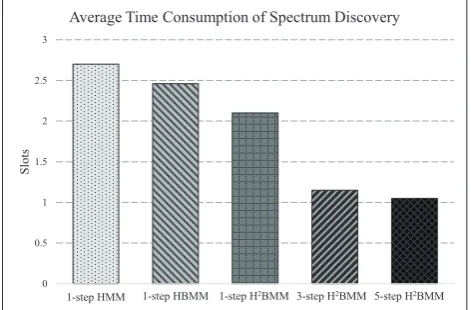
prediction algorithm from 2 to 1, the corresponding time consumption significantly drops from 86% to 43%. In Fig.10, we evaluate the average time consumption on spectrum discovery, which is referred to as the average interval for an SU to find an available channel. The spectrum prediction aims to accelerate the spectrum discovery process. If a channel is predicted to beidle, SUs will access the channel without sensing. Even if the predict results are wrong, it is acceptable as long as SUs exits the channel within the PU’s tolerance period. If the channel is predicted as busy,

0 20 40 60 80 100 120

1-ste_{p HMM} 1-stepHBMM 1-stepH2_BMM3-stepH2_BMM5-stepH2_BMM

R

el

at

iv

e

C

om

pl

ex

it

y

(%

)

Calculation Complexity

Figure 9. Computation Complexity of HMM, HBMM and

H2_BMM

SUs will repeat the discovery process until an idle channel is found. As shown in the figure, H2BMM spends less time than HMM and HBMM to discover an available channel. Besides, multi-step prediction can foresee the channel status of several future slots, which greatly reduces the time consumption of channel detection. Consequently, increasing the prediction steps of H2BMM can further reduce the time consumption on spectrum discovery. In addition, through comparing Figs. 9 and 10, it reveals a trade-off between computation complexity and time consumption on spectrum discovery.

濠瀂濷濸濿瀆 濄激瀆濸瀇瀃澳濛濠濠 濄激瀆濸瀇瀃澳濛濕濠濠 濄激瀆濸瀇瀃澳濛濅_{濕濠濠 濆激瀆瀇濸瀃澳濛}濅_{濕濠濠 濈激瀆瀇濸瀃澳濛}濅_濕濠濠

濦濿瀂瀇瀆 濅濁濊 濅濁濇濉 濅濁濄 濄濁濄濈 濄濁濃濈

0 0.5 1 1.5 2 2.5 3

1-ste_{p HMM} 1-ste_{pHBMM 1-s}te_pH2_{BMM 3-stepH}2_BMM5-stepH2_BMM

Sl

ot

s

Average Time Consumption of Spectrum Discovery

Figure 10. Time Consumption of HMM, HBMM and H2BMM

5.2. Advanced H

BMM vs. H

BMM in a Mobile

CRN

in which each SU detects the PU distributively and shares the sensing information with its neighbors, the Advanced H2BMM collects the sensing data from SUs at the CBS for a centralized spectrum sensing.

2 3 4 5 6 7

The number of SUs

8 9 10

Prediction A

ccuracy

0.65 0.7 0.75 0.8 0.85 0.9

$GYDQFHG _H2_BMM H2_BMM

Figure 11. Prediction accuracy of Advanced H2BMM and

H2_BMM

We first evaluate the prediction accuracy of the Advanced H2BMM and H2BMM in Fig. 11. When a mobile SU moves into the protected area of a PU, both the Advanced H2BMM and H2BMM can update their training matrix based on the new sensing result so that the prediction model can adapt to the new spectrum environment timely. However, as demonstrated in Fig. 11, their prediction accuracies have significant difference. The Advanced H2BMM achieves higher prediction accuracy than the H2BMM benefiting from the centralized spectrum sensing on the CBS. The increased number of SUs sending the sensing data to CBS brings better training on the matrix of H2BMM and improves the prediction accuracy, as illustrated in Fig. 11. By contrast, for H2BMM, the increase of SU number has no evidential impact on the prediction accuracy since each SU conducts the spectrum sensing and prediction independently. The prediction accuracy of H2BMM, therefore, is much lower than that of the advanced H2BMM in a mobile CRN environment.

Fig. 12 compares the false alarm possibilities of H2BMM and Advanced H2BMM. As shown in the figure, when the number of SUs is less than three, the CBS of Advanced H2BMM cannot collect sufficient sensing reports for an accurate channel prediction. Therefore, the Advanced H2BMM has a higher false alarm possibility than H2BMM when the number of SUs is less than 3. When more SUs join the network, the CBS in the Advanced H2BMM collects more sensing information from SUs and becomes better aware of the surrounding channel behavior and hence reduces the

The number of SUs

2 3 4 5 6 7 8 9 10

False Alarm Probability

0.04 0.06 0.08 0.1 0.12 0.14 0.16 0.18 0.2 0.22 0.24

Advanced _H2_BMM

H2_BMM

Figure 12. False alarm of Advanced H2BMM and H2BMM

The number of SUs

2 3 4 5 6 7 8 9 10

Miss Detection Probability

0.06 0.07 0.08 0.09 0.1 0.11 0.12 0.13 0.14 0.15

Advanced_+%00

+_%00

Figure 13. Miss detection of Advanced H2BMM and H2BMM

false alarm probability. The reason why the increase of SU number has no significant effect on H2BMM has been explained in Fig.11.

Advanced High-order Hidden Bivariate Markov Model Based Spectrum Prediction

sensing data and hence to decrease prediction tendency of statusbusy. Similarly, the slight effect of the increase of SU numbers on H2BMM has been explained in Fig.

11.

濠瀂濷濸濿瀆 濛濅濕濠濠澳澻濆激瀆瀇濸瀃澿澳濅瀁濷激瀂瀅濷濸瀅澼 濔濷瀉濴瀁濶濸濷澳濛濅濕濠濠澳澻濆激瀆瀇濸瀃澿澳濅瀁濷激瀂瀅濷濸瀅澼

濦濿瀂瀇瀆 濌濇 濅濆

濠瀂濷濸濿瀆 _{澻濄激瀆瀇濸瀃澿澳濅瀁濷激瀂瀅濷濸瀅澼}濛濅濕濠濠 _{澻濆激瀆瀇濸瀃澿澳濅瀁濷激瀂瀅濷濸瀅澼}濛濅濕濠濠 _{澻濄激瀆瀇濸瀃澿澳濅瀁濷激瀂瀅濷濸瀅澼}濔濷瀉濴瀁濶濸濷澳濛濅濕濠濠 _{澻濆激瀆瀇濸瀃澿澳濅瀁濷激瀂瀅濷濸瀅澼}濔濷瀉濴瀁濶濸濷澳濛濅濕濠濠

濦濿瀂瀇瀆 濌濃 濌濇 濅濃 濅濆

0 10 20 30 40 50 60 70 80 90 100

H2_BMM

(1-step, 2nd-order)

H2_BMM

(3-step, 2nd-order)

Advanced H2_BMM

(1-step, 2nd-order)

Advanced H2_BMM

(3-step, 2nd-order)

R

el

at

iv

e

C

om

pl

ex

it

y

(

%

)

Calculation Complexity

Figure 14. Computation Complexity of Advanced H2BMM and

H2BMM

Now, we compare the computational complexities of Advanced H2BMM and H2BMM in a mobile CRN environment, and show the results in Fig. 14. As we discussed in Fig. 9, the computational complexity is proportional to three parameters, namely, r, m, and k. Therefore, a processor takes a longer time to perform an algorithm with more prediction steps. As observed in Fig. 14, the time consumption of 1-step H2BMM is 90%, which is slightly lower than the 3-step H2BMM. In addition, owing to the enhanced training method, the computational complexities of the 1-step and 3-step Advanced H2BMM are 19% and 23%, respectively, which are much lower than that of the H2_{BMM. Specifically, in the Advanced H}2_BMM,

the training method is improved so that the CBS only needs to calculate the forward and backward probabilities for a small portion of training sequences. By contrast, an SU in H2BMM needs to calculate the forward and backward possibilities of the whole training sequence, which remarkably increases the computational complexity.

The time that H2BMM and Advanced H2BMM spent on discovering the vacant channel is illustrated in Fig.

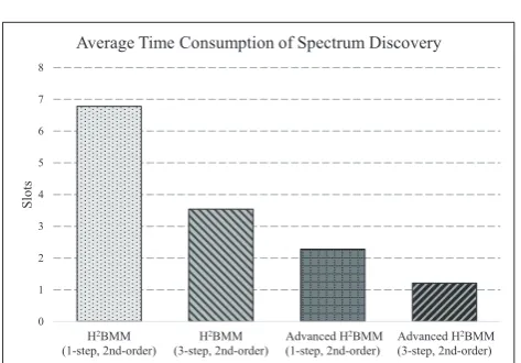
15. Recall that Fig.10indicates less time consumption on spectrum discovery with increased prediction steps. For H2BMM, the time consumptions of 1-step and 3-step prediction are 6.8 and 3.5 slots, respectively, which is accelerated to 2.3 and 1.2 slots in the 1-step and 3-step Advanced H2BMM, respectively. Particularly, the Advanced H2BMM is specially designed for a mobile CRN environment and the H2_{BMM is initially designed}

for a stationary CRN.

To summarize, the Advanced H2_{BMM has superior}

performance than H2_{BMM in a mobile CRN, in terms}

濠瀂濷濸濿瀆 _{澻濄激瀆瀇濸瀃澿澳濅瀁濷激瀂瀅濷濸瀅澼}濛濅濕濠濠 _{澻濆激瀆瀇濸瀃澿澳濅瀁濷激瀂瀅濷濸瀅澼}濛濅濕濠濠 _{澻濄激瀆瀇濸瀃澿澳濅瀁濷激瀂瀅濷濸瀅澼}濔濷瀉濴瀁濶濸濷澳濛濅濕濠濠

濦濿瀂瀇瀆 濉濁濊濋 濆濁濈濇 濅濁濅濋

0 1 2 3 4 5 6 7 8

H2_BMM

(1-step, 2nd-order)

H2_BMM

(3-step, 2nd-order)

Advanced H2_BMM

(1-step, 2nd-order)

Advanced H2_BMM

(3-step, 2nd-order)

Sl

ot

s

Average Time Consumption of Spectrum Discovery

Figure 15. Time Consumption of Advanced H2BMM and

H2BMM

of higher prediction accuracy, smaller false alarm and miss detection probabilities, lower computation complexity and less time consumption on spectrum discover.

6. Conclusion

In this paper, we have proposed a new spectrum pre-diction approach, called the H2_{BMM for CRN. The}

pro-posed approach fully explores the hidden correlation of previous states to make a spectrum prediction. There-fore, it remarkably increases the prediction accuracy compared with the conventional spectrum prediction approaches. To achieve a satisfactory performance in a mobile CRN environment, an Advance H2BMM algo-rithm is also designed through improving the training method of H2BMM. Extensive simulations have been carried out and results verify that the prediction per-formance is significantly improved. The computational complexity and the time consumption for spectrum discovery are evaluated as well.

References

[1] R. Heydari, S. Alirezaee, S. V. Makki, M. Ahmadi, and S. Erfani, “Cognitive radio channel behavior prediction using the hidden Markov model,” inProceedings of the 7th IEEE International Symposium on Telecommunications (IST), 2014, pp. 993–998.

[2] S. H. Sohn, S. J. Jang, and J. M. Kim, “HMM-based adaptive Frequency-hopping cognitive radio system to reduce interference time and to improve throughput,” KSII Transactions on Internet and Information Systems (TIIS), vol. 4, no. 4, pp. 475–490, 2010.

[3] Y. Song and J. Xie, “Prospect: A proactive spectrum handoffframework for cognitive radio ad hoc networks without common control channel,”IEEE Transactions on Mobile Computing, vol. 11, no. 7, pp. 1127–1139, 2012. [4] Z. Lin, X. Jiang, L. Huang, and Y. Yao, “A energy

radio networks,” inProceedings of the 5th IEEE Interna-tional Conference on Wireless Communications, Networking and Mobile Computing, 2009, pp. 1–4.

[5] Y. Zhao, M. Song, C. Xin, and M. Wadhwa, “Spectrum sensing based on Three-State model to accomplish all-level fairness for Co-Existing multiple cognitive radio networks,” in Proceedings of the IEEE Conference on Computer Communications (INFOCOM), 2012, pp. 1782– 1790.

[6] E. Ahmed, L. J. Yao, M. Shiraz, A. Gani, and S. Ali, “Fuzzy-based spectrum handoff and channel selection for cognitive radio networks,” inProceedings of the IEEE International Conference on Computer, Control, Informatics and Its Applications (IC3INA), 2013, pp. 23–28.

[7] X. Xing, T. Jing, W. Cheng, Y. Huo, and X. Cheng, “Spectrum prediction in cognitive radio networks,”IEEE Transactions on Wireless Communications, vol. 20, no. 2, pp. 90–96, 2013.

[8] A. M. Mikaeil, B. Guo, X. Bai, and Z. Wang, “Hidden Markov and Markov switching model for primary user channel state prediction in cognitive radio,” in Proceedings of the 2nd IEEE International Conference on Systems and Informatics (ICSAI), 2014, pp. 854–859. [9] Z. Chen and R. C. Qiu, “Prediction of channel

state for cognitive radio using Higher-order hidden Markov model,” inProceedings of the IEEE SoutheastCon Conference (SECON), 2010, pp. 276–282.

[10] T. Nguyen, B. L. Mark, and Y. Ephraim, “Spectrum sensing using a hidden bivariate Markov model,”IEEE Transactions on Wireless Communications, vol. 12, no. 9, pp. 4582–4591, 2013.

[11] S. Geirhofer, L. Tong, and B. M. Sadler, “Cognitive radios for dynamic spectrum Access-dynamic spectrum access in the time domain: Modeling and exploiting white space,”IEEE Communications Magazine, vol. 45, no. 5, pp. 66–72, 2007.

[12] K. D. Singh, P. Rawat, and J.-M. Bonnin, “Cognitive radio for vehicular ad hoc networks (CR-VANETs): approaches and challenges,” EURASIP Journal on Wireless Communications and Networking, vol. 2014, no. 1, p. 1, 2014.

[13] K. M. Thilina, K. W. Choi, N. Saquib, and E. Hossain, “Machine learning techniques for cooperative spectrum sensing in cognitive radio networks,” IEEE Journal on Selected areas in Communications, vol. 31, no. 11, pp. 2209–2221, 2013.

[14] E. Chatziantoniou, B. Allen, and V. Velisavljevic, “An hmm-based spectrum occupancy predictor for energy

efficient cognitive radio,” inProceedings of the 24th IEEE International Symposium on Personal Indoor and Mobile Radio Communications (PIMRC), 2013, pp. 601–605. [15] C. Chen, G. Vachtsevanos, and M. E. Orchard, “Machine

remaining useful life prediction: An integrated adap-tive Neuro-fuzzy and High-order particle filtering approach,” Elsevier Mechanical Systems and Signal Pro-cessing, vol. 28, pp. 597–607, 2012.

[16] D. Treeumnuk and D. C. Popescu, “Using hidden Markov models to evaluate performance of cooperative spectrum sensing,”IET Communications, vol. 7, no. 17, pp. 1969– 1973, 2013.

[17] R. W. Yan, L. Zhou, and Z. Y. Zhong, “Application of algorithm of hidden Markov model and High-order spectrum in fault diagnosis of power electronic circuit,”

in Advanced Materials Research, vol. 468. Trans Tech

Publ, 2012, pp. 488–491.

[18] B. L. Mark and Y. Ephraim, “An em algorithm for continuous-time bivariate Markov chains,” Elsevier Computational Statistics & Data Analysis, vol. 57, no. 1, pp. 504–517, 2013.

[19] T. Black, B. Kerans, and A. Kerans, “Implementation of hidden Markov model spectrum prediction algorithm,” in Proceedings of the IEEE International Symposium on Communications and Information Technologies (ISCIT), 2012, pp. 280–283.

[20] J. Lan, X. R. Li, V. P. Jilkov, and C. Mu, “Second-order Markov chain based Multiple-model algorithm for maneuvering target tracking,” IEEE Transactions on Aerospace and Electronic Systems, vol. 49, no. 1, pp. 3–19, 2013.

[21] W. Zhao, J. Wang, and H. Lu, “Combining forecasts of electricity consumption in China with TimeVarying weights updated by a High-Order Markov chain model,” Omega International Journal of Management Science, vol. 45, pp. 80–91, 2014.

[22] L. R. Welch, “Hidden Markov models and the Baum-Welch algorithm,” IEEE Information Theory Society Newsletter, vol. 53, no. 4, pp. 10–13, 2003.