Active Information Acquisition With Mobile Robots

(1)

University of Pennsylvania

ScholarlyCommons

Publicly Accessible Penn Dissertations

1-1-2015

Active Information Acquisition With Mobile

Robots

Nikolay Asenov Atanasov

University of Pennsylvania, [email protected]

Follow this and additional works at:

http://repository.upenn.edu/edissertations

Part of the

Computer Sciences Commons,

Electrical and Electronics Commons, and the

Robotics Commons

This paper is posted at ScholarlyCommons.http://repository.upenn.edu/edissertations/1592 For more information, please [email protected].

Recommended Citation

(2)

Active Information Acquisition With Mobile Robots

Abstract

The recent proliferation of sensors and robots has potential to transform fields as diverse as environmental monitoring, security and surveillance, localization and mapping, and structure inspection. One of the great technical challenges in these scenarios is to control the sensors and robots in order to extract accurate information about various physical phenomena autonomously. The goal of this dissertation is to provide a unified approach for active information acquisition with a team of sensing robots. We formulate a decision problem for maximizing relevant information measures, constrained by the motion capabilities and sensing modalities of the robots, and focus on the design of a scalable control strategy for the robot team.

The first part of the dissertation studies the active information acquisition problem in the special case of linear Gaussian sensing and mobility models. We show that the classical principle of separation between estimation and control holds in this case. It enables us to reduce the original stochastic optimal control problem to a deterministic version and to provide an optimal centralized solution. Unfortunately, the complexity of obtaining the optimal solution scales exponentially with the length of the planning horizon and the number of robots. We develop approximation algorithms to manage the complexity in both of these factors and provide theoretical performance guarantees. Applications in gas concentration mapping, joint localization and vehicle tracking in sensor networks, and active multi-robot localization and mapping are presented. Coupled with linearization and model predictive control, our algorithms can even generate adaptive control policies for nonlinear sensing and mobility models.

Linear Gaussian information seeking, however, cannot be applied directly in the presence of sensing nuisances such as missed detections, false alarms, and ambiguous data association or when some sensor observations are discrete (e.g., object classes, medical alarms) or, even worse, when the sensing and target models are entirely unknown. The second part of the dissertation considers these complications in the context of two

applications: active localization from semantic observations (e.g, recognized objects) and radio signal source seeking. The complexity of the target inference problem forces us to resort to greedy planning of the sensor trajectories.

Non-greedy closed-loop information acquisition with general discrete models is achieved in the final part of the dissertation via dynamic programming and Monte Carlo tree search algorithms. Applications in active object recognition and pose estimation are presented. The techniques developed in this thesis offer an effective and scalable approach for controlled information acquisition with multiple sensing robots and have broad applications to environmental monitoring, search and rescue, security and surveillance, localization and mapping, precision agriculture, and structure inspection.

Degree Type Dissertation

Degree Name

Doctor of Philosophy (PhD)

Graduate Group

(3)

First Advisor George J. Pappas

Second Advisor Kostas Daniilidis

Keywords

active object recognition, controlled sensing, control theory, information gathering, robotics, simultaneous localization and mapping

Subject Categories

(4)

ACTIVE INFORMATION ACQUISITION WITH MOBILE ROBOTS

Nikolay Asenov Atanasov

A DISSERTATION

in

Electrical and Systems Engineering

Presented to the Faculties of the University of Pennsylvania in Partial Fulfillment of the Requirements for the

Degree of Doctor of Philosophy

2015

George J. Pappas, Professor of Electrical and Systems Engineering Supervisor of Dissertation

Kostas Daniilidis, Professor of Computer and Information Science Co-Supervisor of Dissertation

Alejandro Ribeiro, Associate Professor of Electrical and Systems Engineering Graduate Group Chairperson

Dissertation Committee:

Daniel D. Lee, Professor of Electrical and Systems Engineering

Vijay Kumar, Professor of Mechanical Engineering and Applied Mechanics

(5)

COPYRIGHT

2015

(6)

(7)

Acknowledgments

This thesis would not have been possible without my advisors, George Pappas, Kostas Daniilidis, and Jerome Le Ny. My deepest thanks go to George for choosing me as his graduate student, teaching me how to think independently, and helping me remember what the point of this huge endeavor is. Thanks to George I learned to communicate my ideas and excite my peers about them. His guidance and support have been my driving force through the years and have shaped my academic identity.

I also thank Kostas for being a source of inspiration, always positive and excited about our research. Our discussions always led to amazing ideas for research problems and inter-esting applications. Most importantly, Kostas motivated me and taught me to enjoy and respect the research process. I am extremely grateful to Jerome for mentoring me and pro-viding support in the difficult moments. Together, we discussed at length both successful and unsuccessful ideas, proofs, and algorithms.

I thank my dissertation committee, Stefano Soatto, Dan Lee, and Vijay Kumar, for putting up with scheduling constraints, wanting to learn about my ideas, and reviewing my work. I thank my co-authors, Bharath Sankaran, Menglong Zhu, Nathan Michael, and Roberto Tron, for helping with a lot of the results and experiments presented in this thesis. I thank Ben Charrow and Phil Dames for our fruitful discussions on information gathering. I thank Hadi, Shahin, Konstantinos, and Omur for the wonderful times we spent doing homework, discussing the challenges of graduate school, and pondering about the future. I had amazing support from my closest friends Petko, Kalin, Rado, Vasil, Yavor, and Kiro. I also thank my undergraduate school advisors Taikang Ning and David Ahlgren for introducing me to engineering research and inspiring me to purse graduate education.

(8)

ABSTRACT

Nikolay A. Atanasov George J. Pappas

Kostas Daniilidis

The recent proliferation of sensors and robots has potential to transform fields as diverse as environmental monitoring, security and surveillance, localization and mapping, and struc-ture inspection. One of the great technical challenges in these scenarios is to control the sensors and robots in order to extract accurate information about various physical phenom-enaautonomously. The goal of this dissertation is to provide a unified approach for active information acquisition with a team of sensing robots. We formulate a decision problem for maximizing relevant information measures, constrained by the motion capabilities and sensing modalities of the robots, and focus on the design of a scalable control strategy for the robot team.

The first part of the dissertation studies the active information acquisition problem in the special case of linear Gaussian sensing and mobility models. We show that the classical principle of separation between estimation and control holds in this case. It enables us to reduce the original stochastic optimal control problem to a deterministic version and to provide an optimal centralized solution. Unfortunately, the complexity of obtaining the optimal solution scales exponentially with the length of the planning horizon and the number of robots. We develop approximation algorithms to manage the complexity in both of these factors and provide theoretical performance guarantees. Applications in gas concentration mapping, joint localization and vehicle tracking in sensor networks, and active multi-robot localization and mapping are presented. Coupled with linearization and model predictive control, our algorithms can even generate adaptive control policies for nonlinear sensing and mobility models.

Linear Gaussian information seeking, however, cannot be applied directly in the presence of sensing nuisances such as missed detections, false alarms, and ambiguous data association or when some sensor observations are discrete (e.g., object classes, medical alarms) or, even worse, when the sensing and target models are entirely unknown. The second part of the dissertation considers these complications in the context of two applications: active localization from semantic observations (e.g, recognized objects) and radio signal source seeking. The complexity of the target inference problem forces us to resort to greedy planning of the sensor trajectories.

(9)

List of Tables

2.1 Suppose that the sensor state isx0, the target covariance is Σ0= 1, and there are two available controlsu(1), u(2). The table shows an example in which the target state is a lot more uncertain afteru(1) _{than after}_u(2) _{but nevertheless} u(1) is considered more informative by the mutual information value func-tion. The problem arises because, while entropy measures the uncertainty in absolute terms, mutual information measures the change in uncertainty af-ter the prediction step. As a result, mutual information encourages controls that create a lot of uncertainty if it can then be reduced significantly via the measurement. In the SLAM context, mutual information might prefer very uncertain (e.g., high velocity) controls even if they provide the same mea-surement information (captured by the sensor matrix M(x) below) as more certain ones.. . . 21

3.1 Comparison of maximum likelihood data association (MLD) and our permanent-based data association approach (PER) with the exact permanent computa-tion (Alg. 6) on the four robot datasets (Fig. 3.15) and the simulacomputa-tions in Fig. 3.10 and Fig. 3.11. Two types of initializations were used: local (L), for which the initial particle set had errors of up to 1mand 30◦, and global (G), for which the initial particle set was uniformly distributed over the whole environment. Number of particles (NP) in thousands, position error (PE), orientation error (OE), and filter update time1(UT), averaged over time, are presented. The first MLD(G) column uses the same number of particles as PER(G), while the second uses a large number in an attempt to improve the performance. . . 73

3.2 Comparison of the average (over 50 simulated environments) performance of the four active-semantic-localization approaches, referenced in Fig. 3.21. The average euclidean distance between the start and the goal positions was 251 m. If the goal was not reached in 1000 iterations, the experiment was terminated. The table presents averages of the number of iterations until termination, the euclidean distance to the goal at termination, the entropy in the particle distributions, and the position and orientation errors with respect to the ground-truth robot trajectory. . . 78

4.1 Simulation results for a bottle detection experiment . . . 113

(13)

4.3 Average precision and relative number of part evaluations versus DPM ob-tained on the bus class from VOC 2007 training set. A grid search over (λf p, λf n)∈ {4,8, . . . ,64} × {4,8, . . . ,64} withλf p ≥λf n is shown. . . 120 4.4 Average precision (AP) and relative number of part evaluations (RNPE) of

DPM versus ADPM on all 20 classes in VOC 2007 and 2010. . . 122

4.5 Average precision (AP), relative number of part evaluations (RNPE), and relative wall-clock time speedup (Speedup) of ADPM versus Cascade on all 20 classes in VOC 2007 and 2010. . . 123

4.6 An example demonstrating the computational time breakdown during infer-ence of ADPM and Cascade on a single image. The number of part evalua-tions (PE) and the inference time (in sec) is recorded for the PCA and the full-dimensional stages. The results are reported once without and once with cache use. The number of part evaluations is independent of caching.. . . . 123

D.1 No missed detections and no clutter: the likelihood p(Z |Yd(x), x) of a set of semantic observations Z is shown for different combinations of m := |Z|

and n:=|Yd(x)|. The dependence of the likelihoods onxis omitted for clarity.157 D.2 No clutter but missed detections are possible: the likelihood p(Z |Yd(x), x)

of a set of semantic observations Z is shown for different combinations of m:=|Z|andn:=|Yd(x)|. The dependence of the likelihoods onxis omitted for clarity. . . 157

D.3 No missed detections but clutter is possible: the likelihoodp(Z|Yd(x), x) of a set of semantic observationsZis shown for different combinations ofm:=|Z|

and n:=|Yd(x)|. The dependence of the likelihoods onxis omitted for clarity.158 D.4 Both missed detections and clutter are possible: the likelihoodp(Z |Yd(x), x)

of a set of semantic observations Z is shown for different combinations of m:=|Z|andn:=|Yd(x)|. The dependence of the likelihoods onxis omitted for clarity. . . 158

(14)

List of Figures

1.1 Autonomous water vehicle tracking radio-emitter-tagged invasive carp species in Minnesota (courtesy of Tokekar et al. 2013 and Choi 2009). . . 2

1.2 Autonomous inspection of the hull integrity of a submerged ship. . . 2

1.3 A military quadrotor patrolling an area of interest. . . 2

1.4 Scheduling communication power, sensor use, and operational parameters in sensor networks is crucial for accurate and efficient tracking of physical phenomena (courtesy of Huber 2009). . . 2

1.5 A robot can improve its localization and environment map by planning an informative trajectory for its future observations (courtesy of Vitus et al. 2012) 2

1.6 Planning the viewpoint of an autonomous camera in order to improve the results of object recognition . . . 2

1.7 To formulate an active information acquisition problem, it is necessary to specify sensor motion models (1.1), target motion models (1.2), sensor ob-servation models (1.3), and an information measure. The task is to design an estimator for the target states and to plan the motion of the sensors in order to improve the estimation performance. The solution should handle heterogeneous sensing systems and should allow for distributed computation and coordination among them. . . 4

(15)

2.1 Forward value iteration (FVI) is a nonmyopic open-loop planning approach which constructs a search tree (right) with branching factor |U | and depth T. It is guaranteed to find the optimal control sequence σ∗ in (2.3) but its complexity is exponential in T (and n). Greedy open-loop planning, on the other hand, keeps only the best node per stage (left) and, hence, has linear complexity in T (and exponential in n) but provides no performance guarantees. . . 20

2.2 Example that greedy planning is worse than nonmyopic planning even for static independent targets and a planning horizon of T = 2. The control sequence chosen by greedy planning is indicated in red, while the optimal two-step sequences are shown in green. . . 20

2.3 Mobile robot equipped with a remote methane leak detector (RMLD) sensor based on tunable diode laser absorption spectroscopy. The RMLD sensor returns a gas concentration measurement in parts-per-million (ppm) inte-grated along the distance in meters (m) traveled by the laser beam (courtesy of Hernandez Bennetts et al. (2013)). . . 29

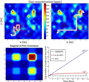
2.4 Comparison of the sensor trajectories (white) obtained by the greedy algo-rithm (top left) and the reduced value iteration algoalgo-rithm (top right) with =∞ and δ = 0 after 40 time steps. A typical realization of the methane field is shown on top, while the diagonal of the prior covariance matrix is shown on the bottom left. The red lines indicate the orientation of the gas sensor during the execution. On the bottom right, the log number of nodes maintained in the search tree by the two approaches is compared to the complete tree maintained by forward value iteration. . . 30

2.5 The Landshark differential-drive robot (left) tracks a mobile target through a wooded area via range and bearing measurements. The plots on the right show the dependence of the sensor performance on the robot speed, the distance to the target, and the target visibility, which can be obstructed by trees. . . 31

2.6 Simulation results from 100 Monte-Carlo runs of the target tracking scenario. Typical realizations are shown on the left. The average root-mean-square error (RMSE) of the estimated target position and velocity is shown on the right, along with the log det of the predicted target covariance on the bottom right.. . . 32

(16)

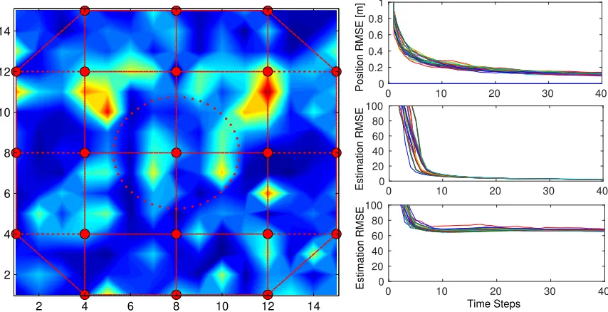
2.8 Two instances of a four-robot active SLAM simulation which demonstrate the estimation quality and the exploration progress in an environment with 200 landmarks. The red dotted curves show the estimated robot trajectories, while the other symbols are described in the caption of Fig. 2.7. The robots have differential drive dynamics with maximum velocity 3m/s, standard de-viations 0.1m/sand 5◦/sin linear and angular velocities, respectively, 10m sensing ranges, 94◦ fields of view, and used range and bearing measurements with standard deviations 0.15 m and 5◦, respectively. See Appendix D.16 Extension 1 for a video of the simulation. . . 37

2.9 The top three plots show the root mean square error (RMSE) in the robot position estimates, the RMSE in the robot orientation estimates, and the entropy of the robot pose estimates, average over 15 repetitions of the four-robot active SLAM scenario in Fig. 2.8. The middle row shows the RMSE in the landmark position estimates, the average entropy in the landmark po-sition estimates, and the entropy of the joint robot-landmark-pose estimate. The last two plots show the percentage of the environment covered by the robots and the number of detected landmarks over time. The robot trajecto-ries were planned using RVI (Alg. 2) with planning horizon T = 12, =∞, and δ = 1.5. The red dotted curves on the last three plots show the per-formance when the trajectories are obtained via a greedy policy (RVI with T = 1). . . 38

2.10 Initial and final (after 20 steps) node locations (red) estimated by the dis-tributed localization algorithm on a randomly generated graph with 300 nodes (blue) and 1288 edges (blue dotted lines) . . . 42

2.11 Root mean squared error of the location estimates obtained from averaging 50 simulated runs of the distributed localization algorithm with randomly generated graphs with 300 nodes (e.g., Fig. 2.10), connectivity radius 10 m, and measurement covariancesEij =I2 . . . 42 2.12 The left plot shows a realization of the vehicle tracking scenario in which

(17)

2.13 Methane emission monitoring via a sensor network. The true (unknown) sensor locations (red nodes), the sensing range (red circle), and a typical re-alization of the methane field are shown on the left. The gas concentration varies from 0 to 800 parts per million (ppm) and the standard deviation of the measurements is 5 ppm. The root mean squared error of the location es-timates and of the field eses-timates obtained from averaging 50 simulated runs of the joint localization and estimation algorithm with continuous sensor ob-servation models are shown in the top two plots on the right (for E_ij =I2). In an additional experiment, the sensors were placed on the boundaries of the cells of the discretized field. As the observation model for each sensor was defined in terms of the proximal environment cells, this made the ob-servation models discontinuous. The bottom right plot illustrates that the concentration estimation error does not vanish when discontinuities are present. 45

3.1 A mobile robot (left) localizes itself within a semantic map of the environ-ment by detecting chairs and doors in images (top middle), obtained from its surroundings. A semantic observation received by the robot (top right) con-sists of a detected class, a detection (confidence) score, and a bearing angle to the detected bounding box. Due to the fact that object recognition misses detections (only one of the two visible chairs is detected) and produces false positives (there is an incorrect door detection), it is appropriate to model the collection of semantic observations via a set with randomly-varying car-dinality. Finally, correct data association between the object detections (top right) and the landmarks on the prior map (bottom right) plays a key role in the robot’s ability to estimate its location. . . 50

3.2 Probability of detecting an object within the sensor field of view (not ac-counting for visibility) . . . 52

3.3 Consider a localization scenario with 16 possible poses, indicated by the arrows on the left-most plot. There are three objects in the environment: a yellow square (class 1), a cyan circle (class 2), and a blue triangle (class 3). Initially, the 16 poses are equally likely (each has weight 1). Suppose that only one set of semantic observations is received. The four plots to the right show how the likelihoods of the 16 locations change, depending on the received set. At each location, the likelihood of the semantic observation set is computed via (3.9) and normalized, so that the sum of the likelihoods is 16. The parameters, used in the semantic observation model, are listed at the top of the plots. For simplicity, the semantic observations here contain only bearing and class information. In the top right plot since the field of view is only 5◦ it is not possible to observe a yellow square at a 45◦ bearing from poses 9−12. Also, since the sensing range is 10 m and there are no missed detections, poses 1−8 and 14−15 are not possible. . . 56

(18)

3.5 The left plot shows a simulation of a 2-D localization scenario with two object classes (circle, square). The prior density of the observer’s pose is represented by the dark red particle set, which is concentrated in 3 locations (green). The observer has a field of view of 360◦ and a sensing range of 4m. The other parameters of the observation model werep0 = 0.73, m0 = 2.7, v0 = 35,Σβ = 4◦, λ = 0.5. The right plot shows the entropy of the observer’s location (in the local frame of reference) conditioned on one set of semantic observations. As the summarized particle set contains only 3 particles, the entropy varies from 0 to 1.099 nats. . . 62

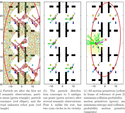
3.6 A simulation of a differential-drive robot employing our active semantic lo-calization approach to reach a goal. The environment contains objects from three classes (square, circle, and triangle) in six areas, divided by the black obstacles. The task of the robot is to localize itself (position and orientation) and reach pose 5, indicated by the green arrow on subplot (b). It has a field of view of 94◦ and a sensing range of 12.5m. The other parameters of the observation model were p0 = 0.73, m0 = 2.7, v0 = 35,Σβ = 5◦, λ= 0.5. The robot had no prior information about its initial pose (subplot (A)). The par-ticle distribution converges to 5 ambiguous locations after several semantic observations because a yellow square and a cyan circle are detected repeat-edly (subplot (B)). The robot plans its motion (using the motion primitives in Fig. 3.4) to minimize the probability of collision and the entropy of its pose, conditioned on 5 future sets of semantic observations (subplot (C)). The description continues in Fig. 3.7. . . 67

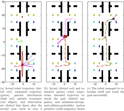
3.7 Continuation of the active semantic localization simulation from Fig. 3.6. The robot recognizes correctly that the best way to disambiguate its pose is to visit the bottom-right area (subplot (A)). At this point, there are only two remaining hypotheses and more weight is starting to concentrate around the true pose. Once the robot considers itself localized (the covariance of the particle set is small), it plans a path to the goal in the top-right area. As there are no landmarks along the hallway, the motion noise causes the uncertainty in the robot pose to increase. Using the entropy-minimization criterion, the robot recognizes that it needs to deviate from its intended path and visit an area with landmarks in order to re-localize (subplot (B)). The robot reaches the goal successfully (subplot (C)). . . 68

3.8 A component of the deformable part model of a chair (top) and scores (bot-tom) from its evaluation on an image (middle) containing four chairs . . . . 70

3.9 Detection score likelihoods obtained from training images . . . 70

3.10 A simulated environment with 45 objects from two classes (yellow squares, blue circles). The plots show the evolution of the particles (red dots), the ground truth trajectory (green), and the estimated trajectory (red). The expected number of clutter detections was set to λ= 2. . . 71

(19)

3.12 A simulated environment with 150 objects from 5 classes (circles, squares, triangles, crosses, and diamonds) in a 25×25 m2 _{area. The plots show the} particles (red dots), the ground truth trajectory (green), and the estimated trajectory (red) for clutter rate λ= 4. . . 71

3.13 Root mean squared error (RMSE) in the pose estimates obtained from the semantic localization algorithm after 50 simulated runs of the scenario in Fig. 3.10 . . . 71

3.14 Root mean squared error (RMSE) between the pose estimates from semantic localization and from lidar-based geometric localization obtained from four real experiments . . . 71

3.15 Robot trajectories estimated by lidar-based geometric localization (red), image-based semantic localization (blue), and odometry (green) in a real experi-ment. The starting position, the door locations, and the chair locations are denoted by the red cross, the yellow squares, and the cyan circles, respec-tively. See Appendix D.16 Extension 2 for more details. . . 72

3.16 Particle filter evolution (bottom) and object detections (top) during a real semantic localization experiment . . . 72

3.17 Tango phone trajectory (red) estimated via semantic localization in a real experiment. The semantic map contains doors (yellow squares), red chairs (cyan circles), and brown chairs (blue triangles). Ground-truth information was not available for this experiment. See Appendix D.16 Extension 4 for more details. . . 74

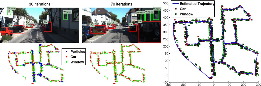
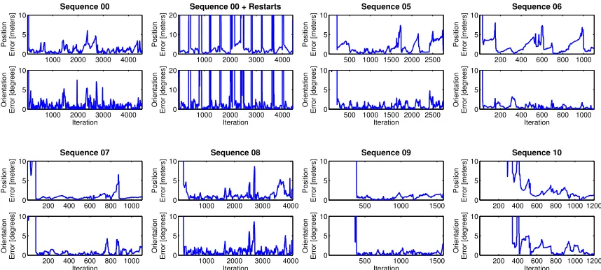
3.18 Vehicle trajectory estimated via global semantic localization on sequence 00 from the KITTI visual odometry dataset. The left and middle plots show two images with car and window detections and the corresponding particle distributions in the semantic map. The plot on the right shows the semantic map and the trajectory, recovered after unique localization (iteration 70). See Appendix D.16 Extensions 5 and 6 for more details. . . 75

3.19 Position (euclidean distance) and orientation errors of the vehicle trajectories recovered via global semantic localization on sequences{00,05,06,07,08,09,10}

from the KITTI visual odometry dataset. The plot, titled “Sequence 00 + Restarts”, shows results from an experiment in which the localization was restarted every 400 iterations. Appendix D.16 Extensions 5 - 13 provide videos of all experiments. . . 76

(20)

3.21 The left plot shows the trajectories, followed by four different active-semantic-localization approaches, which localize and lead a differential-drive robot to a goal pose in a simulated environment containing 300 objects from 3 classes (yellow square, cyan circle, blue triangle). The initial particle distribution is shown by the black dots. The four methods are: (1) ASL: active semantic localization presented in Sec. 3.1.5, (2) RND: chooses motion primitives at random, (3) MIN: chooses the motion primitive that drives the particle mean closest to the closest landmark, (4) BEM: bearing-only entropy minimization (see text for details). The right plot shows the particle-distribution entropies along the trajectories associated with each method. . . 77

3.22 A differential-drive Scarab robot equipped with a XBee-PRO RF module. . 89

3.23 A path followed by the robot after 20 iterations of the random-direction stochastic approximation algorithm (3.29) in an obstacle-free environment is shown on the left. The blue circles indicate positions at which the robot measured the signal strength. The white dots indicate the starting and final positions of the robot and are 21.85 m and 1.47 m away, respectively, from the actual position of the source. The right plot shows the final distance to the source calculated over 50 independent replications. The source was 21.85 m away initially. The bars show one standard deviation. . . 90

3.24 A path followed by the robot after 20 iterations of the random-direction stochastic approximation algorithm (3.29) in an environment with obstacles is shown on the left. The white dots indicate the starting and the final positions. The seeker and the source were 17.85 m apart initially and 0.75 m apart in the end. The distance to the source calculated over 50 independent replications of the algorithm is shown on the right. The initial distance from the source was 17.85 m. The bars show one standard deviation from the mean. 90

3.25 Path followed by the robot after 10 iterations of the random-direction stochas-tic approximation algorithm (3.29) in a real environment. The seeker was 17.9 m away from the source initially. The red circle shows the final estimate of the source location and is 2.2 m away from the actual one, denoted by the blue cross. The received-signal-strength measurement history is shown on the right. See Appendix D.16 Extension 15 for a video of the experiment. 91

(21)

3.27 The paths followed by the sensors after 30 iterations of the model-free source-seeking algorithm in an obstacle-free environment. The white circles indicate sensor 1’s estimates of the source position over time. The plots on the right show the average error of the source position estimates and its standard deviation averaged over 50 independent repetitions. . . 93

4.1 Database of object models constructed using kinect fusion (Newcombe et al., 2011) and an example of a scene used to evaluate our framework in simulation.103

4.2 An example set of hypotheses about the class and orientation of an unknown object . . . 104

4.3 Setup for the active object recognition problem. The camera position is restricted to a set of viewpoints (green) on a sphere centered at the object’s location. The task is to choose a camera control policy, which minimizes the movement cost and the probability of misclassification. . . 105

4.4 The sensor position is restricted to a set of points on a sphere centered at the location of the object. Its orientation is fixed so that it points at the centroid of the object. A point cloud is obtained at each viewpoint, key points are selected, and local features are extracted (top right). The features are used to construct a VP-Tree (bottom right). . . 106

4.5 Confusion matrix (left) for all classes in the VP-Tree. A class is formed from all views associated with an object. The effect of signal noise on the classification accuracy of the VP-Tree is shown on the right. . . 107

4.6 Observation model obtained with seven hypotheses for the Handlebottle

model and the planning viewpoints used in the simulation experiments (Sec. 4.4.4). Given a new VP-Tree observation zt+1 from the viewpoint xt+1, the observation model is used to determine the data likelihood of the observation and to update the hypotheses’ prior by applying Bayes rule. . . 109

4.7 Twenty five hypotheses (red dotted lines) were used to decide on the orienta-tion of a Watercan. The left plot shows the error in the orientaorienta-tion estimates as the ground truth orientation varies. The error averaged over the ground truth roll, the hypotheses over the object’s yaw (blue dots), and the overall average error (red line) are shown on the right. . . 114

4.8 An example of the experimental setup (left), which contains two instances of the object of interest (Handlebottle). A PR2 robot with an Asus Xtion RGB-D camera attached to the right wrist (middle) employs the nonmyopic view planning approach for active object classification and pose estimation. In the robot’s understanding of the scene (right), the object which is currently under evaluation is colored yellow. Once the system makes a decision about an object, it is colored green if it is of interest, i.e. in I, and red otherwise. Hypothesis H(0◦) (Handlebottle with yaw 0◦) was chosen correctly for the green object. See the video in Appendix D.16 Extension 16 for more details. 115

(22)

4.10 Active DPM Inference: A deformable part model trained on the PASCAL VOC 2007 horse class is shown with colored root and parts in the first column. The second column contains an input image and the original DPM scores as a baseline. The rest of the columns illustrate the ADPM inference which proceeds in rounds. The foreground probability of a horse being present is maintained at each image location (top row) and is updated sequentially based on the responses of the part filters (high values are red; low values are blue). A policy (learned offline) is used to select the best sequence of parts to apply at different locations. The bottom row shows the part filters applied at consecutive rounds with colors corresponding to the parts on the left. The policy decides to stop the inference at each location based on the confidence of foreground. As a result, the complete sequence of part filters is evaluated at very few locations, leading to a significant speed-up versus the traditional DPM inference. Our experiments show that the accuracy remains unaffected. 119

4.11 Average precision and relative number of part evaluations versus DPM as a function of the parameter λ= λf n =λf p on a log scale. The curves are reported on the bus class from the VOC 2007training set. . . 121

4.12 Illustration of the ADPM inference process on a car example. The DPM model with colored root and parts is shown on the left. The top row on the right consists of the input image and the evolution of the positive label probabilitypt(⊕) fort∈ {1,2,3,4}(high values are red; low values are blue). The bottom row consists of the full DPMscore(q) and a visualization of the parts applied at different locations at timet. The pixel colors correspond to the part colors on the left. In this example, despite the car being heavily occluded, ADPM converges to the correct location after four iterations. For more examples see the video in Appendix D.16 Extension 17. . . 122

(23)

Chapter 1 Introduction

1.1 Motivation

The heart of data-enabled science is the extraction and interpretation of information residing in dynamic hard-to-predict phenomena. Classically, information is collected by static sen-sors and is summarized in spatiotemporal models, represented in the language of Bayesian filters and graphical models. The stance of this thesis is that going beyond static data collection will enable intelligent sampling and will produce higher-fidelity models efficiently. Autonomous sensor deployments are also adaptable to environment conditions and will re-duce human supervision and allow access to dangerous areas. The effective coordination of mobile sensing resources relies on and aims at improving the models produced at the inference level. Due to this coupling, information-gathering problems are quite challenging and necessitate the development of new principled approaches for dealing with the underly-ing complexity. A small tweak in the existunderly-ing body of work is unlikely to yield the desired results. In particular, there is a need for breakthroughs in hierarchical representations, dis-tributed inference, and adaptive planning algorithms, which are scalable both in the length of the planning horizon and in the number of sensors and can handle heterogeneity both in the environment models and in the vehicle dynamics. In exchange, the rewards are com-pelling. Distributing the estimation and control will allow robust coordination of numerous intelligent systems. Heterogeneity will enable collaboration among water, ground, and air resources with various sensing capabilities, thereby dramatically improving the awareness of the sensor team at metric, topological, and semantic levels. Such developments will have a tremendous impact in the following fields:

• Environmental monitoring (Fig. 1.1): air, water, and soil quality, temperature, pres-sure, magnetic forces, chemical concentration, diffusivity, bio-diversity

• Agriculture

• Construction and structure inspection (Fig. 1.2)

• Security and surveillance (Fig. 1.3 & Fig. 1.4)

• Search and rescue operations

(24)

• Localization and mapping (Fig. 1.5)

• Mining

• Space exploration

Therefore, the focus of this dissertation is on active information acquisition with mobile robots and configurable sensing systems. In the next section, we capture the characteristics of the aforementioned scenarios in a precise problem formulation. The objective is to design a scalable control strategy for the robot team in order to tracking evolving phenomena of interest accurately and efficiently.

Figure 1.1: Autonomous water vehicle tracking radio-emitter-tagged invasive carp species in Minnesota (courtesy ofTokekar et al. 2013andChoi 2009).

Figure 1.2: Autonomous inspection of the hull integrity of a submerged ship.

Figure 1.3: A military quadrotor pa-trolling an area of interest.

Figure 1.4: Scheduling communication power, sensor use, and operational parameters in sensor networks is crucial for accurate and efficient tracking of physical phenomena (cour-tesy ofHuber 2009).

Figure 1.5: A robot can improve its localization and envi-ronment map by planning an informative trajectory for its future observations (courtesy ofVitus et al. 2012)

(25)

1.2 The Active Information Acquisition Problem

Information acquisition is the process of estimating the state of an observed system of inter-est by utilizing the available sensing modalities. Consequently, approaches from inter-estimation theory, such as filtering, smoothing, and belief propagation, form the basis of information acquisition. Active information acquisition, on the other hand, is the process of planning future trajectories and configurations for the sensing systems, over multiple time steps, in order to improve the performance of the estimation process. It couples the estimation prob-lem with a stochastic control probprob-lem, which requires making decisions based on anticipated, not-yet-known sensor measurements.

The starting point of an active information gathering algorithm is a collection of three dynamical models which capture mathematically the degrees of freedom of our sensors, the evolution of the physical process, and relationship between the sensor observations and the target process. Having designed these models, one can proceed with the construction of an estimator which uses the sensor observations to refine the knowledge about the state of the underlying physical process. The final step is to plan the motion and configurations of the sensors in order to collect maximally-informative observations, thus optimizing the estimation process. This requires a proper choice of a reward function to judge the infor-mativeness of the planned sensor trajectories. Fig. 1.7 presents an overview of the active information acquisition process.

Proceeding more formally, consider a team of n mobile sensors with states xi,t, i =

1, . . . , n at time t and dynamics governed by the following discrete-time continuous-state

sensor motion model:

xi,t+1=fi(xi,t, ui,t,noise), (1.1)

whereui,t is the control input. To simplify notation, denote the collection of all sensor states

by xt:= [xT1,t· · ·xTn,t]T, the collection of all inputs byut:= [uT1,t· · ·uTn,t]T, and the combined

sensor motion model by xt+1 =f(xt, ut,noise). In many applications, the sensor mobility

is due to the fact that the sensors are mounted on a vehicle or a robot. For example, the kinematics of a ground robot with nonholonomic (car-like) constraints can be described by a differential-drive model (AppendixB.1).

The task of the sensors is to track the evolution of a collection of targets (e.g., mobile vehicles, visual landmarks, radio transmitters, gas concentration in different regions of the environment, etc.) with joint stateyt. The target evolution is governed by a target motion model:

yt+1=a(yt,noise). (1.2)

For example, the behavior of a mobile target in tracking scenarios is often described by a constant-velocity motion model (Appendix B.2).

Each sensor receives measurements zi,t of the targets, governed by the following sensor observation model:

zi,t =hi(xi,t, yt,noise). (1.3)

Again, to simplify notation, we usezt:= [z1T,t· · ·zn,tT ]T and denote the combined observation

model by zt=h(xt, yt,noise). Some widely-used sensing models are provided in Appendix

(26)

Figure 1.7: To formulate an active information acquisition problem, it is necessary to specify sensor motion models (1.1), target motion models (1.2), sensor observation models (1.3), and an information measure. The task is to design an estimator for the target states and to plan the motion of the sensors in order to improve the estimation performance. The solution should handle heterogeneous sensing systems and should allow for distributed computation and coordination among them.

(AppendixB.5), and an odometry sensor, such as a combination of an inertial measurement unit (IMU) and wheel encoders, can be modeled as a 2-D relative-pose sensor (Appendix

B.6) because it estimates the transformation between two successive robot poses. Often times, especially for more complicated systems, the motion and observation models can be learned from training data via machine learning and system identification techniques.

In addition to the sensor and target models described above, there are several other considerations for specifying the active information acquisition problem. We state the problem formally first and discuss the additional ingredients afterwards.

Problem (Active Information Acquisition). Given initial sensor states x0, a prior p0 on

the target states, and a planning horizon T < ∞, choose control policies µt := {µi,t | i=

1, . . . , n} fort= 0, . . . , T−1 that map the history of control inputs and sensor observations to new control inputs for the sensors and aim to maximize information about the target:

max

µ0:T−1

I(y1:T, x1:T, z1:T)

s.t. xt+1=f(xt, µt,noise) yt+1 =a(yt,noise) zt=h(xt, yt,noise)

(1.4)

where I is an information measure.

Many variants of the above problem can be considered (e.g., linear or nonlinear models

(27)

or to estimate unknown parameters of spatially-distributed systems (Rafajlowicz 1986). If the maneuverability of the sensor is constrained, the future behavior of the target has to be anticipated at an early stage in order to obtaining good sensor positioning. We discuss the ingredients which determine the type of active information acquisition problem below.

Target state estimator

Before we even consider planning the motion of the sensors, we need to design an estimator which uses sensor observations to refine the knowledge about the target. As stated in the problem formulation, we are given a prior probability density (or mass) function (pdf) p0

of the target states y0. The task of the estimator is to propagate the pdf pt over time by

using incoming measurements and the motion and observation models. This is precisely the topic of estimation theory and is addressed by filtering (Huber 2009), smoothing (Kaess 2008), or graphical-model inference (Koller and Friedman 2009) techniques. Appendix C

introduces Bayesian filtering and two of the most successful filters in practice - the Kalman filter (AppendixC.1) and the particle filter (AppendixC.3). These filters, along with some more sophisticated variants, are employed for target estimation in this dissertation.

While planning the sensor motion in problem (1.4), a target estimator has to be exe-cuted multiple times to predict the target behavior, especially for long planning horizons. Hence, the more accurate and complex the employed estimator is, the more computationally-demanding and informative the resulting sensor control policies are. Here, it is important to note that the estimator employed for informative planning does not necessarily have to be the same as the one used for inferring the target state when the actual sensor measurements arrive. A practical way to trade off estimation accuracy and computational resources is to use a high-fidelty estimator during inference (since it has to be executed only once per time step) and a less-complex estimator during planning (since it has to be executed many times while solving problem (1.4)). This might be suboptimal but in practice inference needs to be precise, while planning needs to be fast!

Information measure

The target state estimator provides a (usually finite-dimensional) representation of the target pdf pt that can be used to judge the uncertainty (or information) contained in the

current estimate of the target state. The information measureI(y1:T, x1:T, z1:T) in problem

(1.4) does precisely this - it captures the improvement in the target estimate along different sensor trajectories. For example, we can think of the active information acquisition problem as planning a sensor trajectory that will improve the uncertainty (captured by the covariance matrix) of a Kalman filter the most. Hence, the design of an appropriate information measure is an important consideration for active information gathering. This thesis relies on information theory for suitable candidates such as conditional entropy H(y1:T, x1:T |z1:T),

mutual informationI(y1:T, x1:T;z1:T), and probability of error (see AppendixAfor details).

(28)

pdf but might be notoriously difficult to evaluate for multimodal distributions (Ch. 3). In the latter case, it might be more appropriate to use a measure such as Cauchy-Schwarz mutual information (Charrow et al. 2015, Kampa et al. 2011) or quadratic R´enyi entropy (R´enyi 1961, Carrillo et al. 2015a), which have a closed-form expression for mixtures of Gaussians.

Planning horizon

Another determinant of the complexity of the active information acquisition problem is the length T of the planning horizon. If the horizon is T = 1, we obtain a (greedy) next-best-sensor-view problem. At the other extreme, ifT =∞, we get a persistent monitoring problem, in which attention can be restricted to periodic sensor trajectories (Zhao et al. 2014). In Ch. 2, we will observe that, for T <∞, the complexity of the active information acquisition problem grows exponentially with the length of the planning horizon. Hence, it is desirable to investigate approximate solutions that mitigate this complexity but retain some performance guarantees. Finally, if the planning horizonT is subject to optimization (not fixed), we get an optimal stopping problem, which will be considered in Ch. 4.

Optimization type

The active information acquisition problem has strong relations to stochastic optimal control for dynamic systems. In fact, in its most general form (1.4) it can be considered an instance of a partially observable Markov decision process (POMDP, Bertsekas (1995)). However, instead of assuming a general value function (as done in POMDP planning), this thesis exploits the properties of the information measure to offer a more scalable, efficient, and precise solution than what is offered by a general POMDP solver.

As mentioned before, one of the factors that determines the complexity of the planning problem is the horizon lengthT. Perhaps, the easiest instance of the problem is to compute a greedy control policy, i.e., one that quantifies the sensing performance only at the next time step. A solution to a longer-horizon problem can be constructed by committing to the greedy policy in the first step and solving a series of such single-step optimizations. We call this approach greedy planning. This is in contrast with nonmyopic planning which solves (1.4) directly with a longer planning horizon (T >1).

Planning approaches can also differ in their adaptability to future measurements. Open-loop planning fixes some expected values for the future measurements and computes a

sequenceof controls assuming that these most-likely observations will happen. At run time, the same sequence of sensor inputs will be executed regardless of the actual measurement realizations. Closed-loopplanning, on the other hand, computes a sequence of functions (i.e., a policy) which map to an appropriate control input depending on the actual measurement realizations. As a result, the closed-loop policy is adaptable to the actual measurements at run time.

We can use an example to clarify the distinctions among the four types of optimization: greedy closed-loop, nonmyopic closed-loop, greedy open-loop, and nonmyopic open-loop. Consider a sensing system that can be in two states x ∈ {0,1} and the control input

u ∈ {0,1} selects the system state without noise. Suppose that the sensor is binary too,

(29)

(a) nonmyopic closed-loop planning (b) greedy closed-loop planning

(c) nonmyopic open-loop planning (d) greedy open-loop planning

Figure 1.8: Comparison among greedy, nonmyopic, open-loop, and closed-loop planning variants. The blue nodes represent the sensor states in a tree of depth 2, corresponding to the planning horizon length. Nonmyopic closed-loop planning considers all possible combinations of future observations z and controlsu. Nonmyopic open-loop planning, on the other hand, commits to some most-likely observations beforehand and only considers the possible control input variations. The corresponding greedy versions commit to a control policy (or input) at the first level of the tree and then explore only the subtrees starting from it. Intuitively, we can expect nonmyopic closed-loop planning to be the most computationally demanding, while greedy open-loop planning to be the least.

optimize the sensor performance, we need to explore a tree of possible control inputs and measurement realizations of depth T = 2. See Fig. 1.8 for a visualization. Nonmyopic closed-loop planning considers all possible control inputs, all possible measurement real-izations, and the whole planning horizon (Fig. 1.8(a)). Greedy closed-loop planning, on the other hand, explores a tree of depth 1 first and commits to a single-step control policy. Afterwards, it explores the second level of the tree but, due to committing early, some of the nodes are not reachable (Fig. 1.8(b)). Nonmyopic open-loop planning explores the whole tree but commits to some most-likely observations beforehand. Essentially, it removes all branching possibilities associated with the measurements and then searches the tree for a control sequence, rather than a function of the possible measurements (Fig. 1.8(c)). Finally, greedy open-loop planning commits to some most-likely observations and explores a tree of depth 1 first. It commits to a single control input (not policy) and then explores only the subtree starting from it (Fig. 1.8(d)).

(30)

computation-ally demanding approach but provides the best sensor performance, since it explores all future possibilities. At the other extreme, greedy open-loop planning is the fastest to com-pute but might ignore lots of possible future realizations. It has been shown in the literature (Williams 2007, Ch.3.5.1) that greedy closed-loop planning can be arbitrarily worse than nonmyopic closed-loop planning. Greedy closed-loop planning may be competitive with nonmyopic open-loop planning in some settings (Williams 2007, Thm.3.8). Further, non-myopic open-loop planning may be arbitrarily worse than nonnon-myopic closed-loop planning (Hollinger et al. 2013a, Thm.1). Interestingly, we will see in Ch. 2 that active information acquisition with linear Gaussian sensing and motion models is anexception. In other words, there is no gain in the performance of closed-loop planning over that of open-loop planning. However, we will also show that greedy planning is worse than nonmyopic planning even for static independent targets (Ch. 2).

A compromise between open-loop and closed-loop planning is open-loop feedback con-trol (Bertsekas 1995). Like in open-loop planning, future measurements are fixed at some most-likely values but when an actual measurement arrives it is used for computing an updated plan. This idea of planning an open-loop sequence, applying the first control in-put, and replanning after the next observation is also known as receding horizon control or model predictive control (Morari and Lee 1999, Rawlings and Mayne 2009). It can be shown that open-loop feedback control is no worse than open-loop planning but again its performance may be arbitrarily worse than that of closed-loop planning (Bertsekas 1995). We will combine nonmyopic open-loop planning with model predictive control in Ch. 2to obtain an adaptive control policy for nonlinear sensor and target models.

1.3 Related Work

Since many variants of the general formulation in (1.4) have been studied, this section provides only a high-level overview of the related work. The closest approaches will be discussed in more detail within the specific context of the later chapters.

The idea of optimizing the performance of configurable sensing systems dates back to the 60’s (Meier et al. 1967,Athans 1972). Earlier approaches to active information acquisition considered stateless sensor systems (systems whose internal state is not affected by the control and all controls are available at all times) in problems such as sensor selection (Joshi and Boyd 2009), sensor placement (Krause 2008), sensor scheduling (Gupta et al. 2006,Le Ny et al. 2011,Vitus et al. 2012), and active hypothesis testing (Naghshvar and Javidi 2013b,a,Nitinawarat and Veeravalli 2013a,Nitinawarat et al. 2013).

More recently, attention has shifted to dynamic sensors and complex estimation tech-niques but, typically, greedy control. Examples include range-only target tracking (Mart´ınez and Bullo 2006), the next-best-view problem in active object recognition (Bajcsy 1988,

(31)

(Hoffmann and Tomlin 2010, Julian et al. 2012, Meyer et al. 2014, Dames and Kumar 2013).

As may be expected, non-greedy active information acquisition is an even harder problem (Le Ny 2008). Ryan and Karl Hedrick(2010) consider the impact of multiple measurements over time in the context of information-theoretic mobile target tracking. Mutual information is approximated using Monte Carlo sampling, which leads to a computationally-expensive algorithm. There is a line of work which alleviates the complexity, associated with longer planning horizons, by assuming linear Gaussian sensing models. Examples include sampling-based (Hollinger and Sukhatme 2013,2014,Lan and Schwager 2013), search-based (Le Ny and Pappas 2009,Atanasov et al. 2014a) and submodularity-based approaches (Singh et al. 2009a,b) for open-loop informative planning in Gaussian random fields (Le Ny and Pappas 2009) and Gaussian process models (Marchant and Ramos 2014). Finally, there does not exist a specialized information planner for nonmyopic closed-loop information gathering with general sensing models (non-Gaussian and non-linear). However, the problem is an instance of a partially-observable Markov decision process and work in POMDP planning (Kaelbling and Lozano-Pérez 2013, Kurniawati et al. 2008, Silver and Veness 2010) and belief-space planning (Hauser 2011,Indelman et al. 2014,Prentice and Roy 2009) is relevant. Important applications of active information acquisition include environmental mon-itoring (Choi 2009, Tokekar 2014), search and rescue (Kumar et al. 2004), security and surveillance (Rybski et al. 2000), structure inspection (Hollinger et al. 2013b), source seek-ing (Zhang et al. 2007,Ghods and Kristić 2011,Stanković and Stipanović 2010, Atanasov et al. 2015b), active perception (Denzler and Brown 2002, Valente et al. 2014, Atanasov et al. 2014b), and active simultaneous localization and mapping (SLAM, Carlone et al.

(2014),Sim and Roy (2005),Kontitsis et al. (2013),Atanasov et al. (2015a)).

1.4 Outline and Contributions

The long-term goals of the work described in this dissertation are:

• Improved representation: Before considering controlled information acquisition, it is necessary to establish reliable target modeling and estimation techniques. In most cases, traditional tools such as Gaussian processes, Bayes Nets, and Kalman and particle filters suffice. However, it is desirable to develop inference methods that can simultaneously handle continuous variables (e.g., target poses), discrete variables (e.g., target classes), and sensing nuisances, such as false and missed detections and ambiguous data association (the mapping between received measurements and visible targets).

(32)

air and ground vehicles, linear and nonlinear sensing models, discrete and continuous measurements, static and mobile targets).

• Scalability: Both the inference and the information-planning approaches need to scale well with respect to the length of the planning horizon and the number of sensing systems. This inevitably leads to considerations for distributed estimation and control techniques that facilitate coordination and collaboration among the sensing systems.

• Experimental validation: The proposed algorithms should be validated in real-world experiments and should be compared with alternative approaches.

Below is a brief overview of the chapters and their contributions with respect to the existing work and the goals listed above.

Chapter 2: Dynamic optimization over a long time horizon is required to obtain a sensor control policy that anticipates the target evolution and avoids local minima of the infor-mation measure. To deal with the increasing complexity of longer planning horizons, this chapter takes advantage of two key observations:

• An active information acquisition problem with nonlinear non-Gaussian motion and observation models can be converted into a linear Gaussian one via statistical lin-earization as long as the motion and observation models are continuous.

• The classical separation principle (Athans 1972,Meier et al. 1967) between estimation and control holds for the linear Gaussian Active Information Acquisition problem. As a result, the optimal estimator is the Kalman filter and the problem can be reduced from a stochastic optimal control problem to a deterministic one, where open-loop policies achieve the optimal solution. Still, the complexity of computing the optimal nonmyopic open-loop policy scales exponentially with the planning horizonT and the number of sensorsn.

The chapter makes the following contributions.

• We prove the separation principle holds for the linear Gaussian Active Information Acquisition problem.

• We develop an approximation algorithm with finite-time suboptimality guarantees for nonmyopic open-loop planning that manages the complexity inT. The algorithm can be used in combination with model predictive control to produce an adaptive policy for nonlinear motion and observation models.

• We propose a decentralized control scheme to achieve linear complexity in the number of sensors n. We prove that the approach obtains at least 50% of the (mutual) information obtained by the optimal centralized solution.

(33)

• We present applications in methane emission monitoring, mobile vehicle tracking, distributed localization in sensor networks, and active multi-robot simultaneous lo-calization and mapping.

Chapter 3: In the presence of sensing nuisances, such as missed detections and false alarms, and discrete or strongly nonlinear observation models, the conversion into a linear Gaussian information gathering problem is of limited fidelity. Even worse, sometimes the target motion model and sensor observation model are completely unknown. The classical estimation techniques, such as the Kalman filter and the particle filter, are not sufficient here. The focus of this chapter is on target inference techniques that can deal with such difficult situations. Due to the complexity of the inference process, the control in this chapter is greedy. We make the following contributions.

• We develop a sensor observation model for set-valued measurements which incorpo-rates missed detections, false alarms, and data association.

• We prove that obtaining the likelihood of a set-valued sensor observation is equivalent to a matrix permanent computation. This allows a polynomial-time approximation to a Bayes filter with set-valued observations.

• We develop a stochastic gradient ascent scheme for multi-sensor information gathering with unknown sensor observation and target motion models. Gaussian radial basis functions are used to calculate finite-difference weights which approximate the gradient of the measured signal. We prove that our approach converges to a local maximum of the measured signal.

• We present applications in vehicle localization in residential areas using semantically meaningful landmarks, global localization of Google’s Project Tango phone (Google ATAP group 2014), active robot localization using object detections, and wireless radio source localization.

Chapter 4: The simplest case in which the linearization technique of Ch. 2 cannot be applied is when some measurement or state variables are discrete. For example, we face such complications in active vision problems where scene labels and object classes are dis-crete. Unfortunately, removing the linear Gaussian assumptions invalidates the separation principle and closed-loop planning is needed to solve the original stochastic optimal control problem (1.4). Unlike Ch. 3which uses greedy planning, this chapter focuses on nonmyopic closed-loop planning for information gathering in discrete state and measurement spaces. The chapter makes the following contributions.

• We formulate an active information acquisition problem with motion and observation models described by arbitrary probability mass functions. This formulation is par-ticularly suitable for active object recognition, classification, and hypothesis testing problems.

(34)

with the size of the state and measurement spaces. To provide scalability, we also propose an approximate algorithm based on Monte Carlo tree search (Browne et al. 2012) with a rollout policy that exploits the structure of the information measure.

• We demonstrate that these ideas can improve object classification and pose estimation with a mobile camera and can also speed up object recognition with deformable part models (Felzenszwalb et al. 2010b).

(35)

Chapter 2 Nonmyopic Information Acquisition

with Linear Gaussian Models

Sensor management (Hero III and Cochran 2011) offers a formal methodology to control the degrees of freedom of sensing systems in order to improve the information acquisition process. The earliest approaches date back to the 60’s (Meier et al. 1967, Athans 1972). Efficient nonmyopic planning approaches have been proposed for sensors without internal states in the context of sensor placement and scheduling (Gupta et al. 2006,Le Ny et al. 2011, Krause et al. 2008, Krause 2008, Vitus et al. 2012, Williams 2007, Joshi and Boyd 2009). However, when it comes to optimizing the trajectories of mobile sensors, which possess internal states, the approaches are often greedy and rarely provide performance guarantees. The main complication is that the evolution of the sensor states depends on the control inputs and affects the measurements in the long run. Concretely, whereas in radar management a sensor can switch instantaneously between targets (Krishnamurthy and Evans 2001), a feasible and informative path needs to be designed for a sensing robot (Singh et al. 2009a). Due to this complication, most approaches for information gathering with mobile sensors are greedy (Grocholsky 2002,Chung et al. 2006) or use short planning horizons (Kreucher 2005,Huber 2009). However, it is precisely the presence of internal states that makes multi-step optimization important. The behavior of the observed phenomenon needs to be predicted at an early stage to facilitate effective control of the mobile sensor.

This chapter exploits a key insight that under linear Gaussian assumptions on the target and observation models the active information acquisition problem (1.4) can be formulated as a deterministic optimal control problem (Le Ny and Pappas 2009). As a result, in-formative sensing paths can be computed via open-loop planning and there is no loss in performance with respect to closed-loop planning. The advantage is that the search space of a deterministic control problem is significantly smaller than the stochastic version. The problem can be solved forward in time, considering reachable states only, instead of discretiz-ing the high-dimensional search space as required by backward value iteration (Bertsekas 1995). Still, the complexity of the optimal nonmyopic open-loop solution turns out to be exponential in both the planning horizonT and the number of sensorsn.

(36)

tra-jectories from the search space. We prove that this results in bounded suboptimality with respect to the optimal centralized solution and allows much faster nonmyopic planning. Coupled with linearization and model predictive control, this approach can even generate adaptive policies for non-linear motion and observation models. Our work can be consid-ered a search-based method for planning in information space. Related work in this area includes (Zhou 2012,Vander Hook et al. 2014,Le Ny and Pappas 2009). Some successful approaches for open-loop informative planning rely on a submodular function to quantify the informativeness of the sensor paths (Singh et al. 2009a,b). The sensing locations are partitioned into independent clusters. Submodularity is used to greedily select informative locations within clusters. An orienteering problem is solved to choose the sequence of clus-ters to visit. The drawback is that within clusclus-ters the movement of the sensor is restricted to a graph, essentially ignoring the sensor dynamics. As a result, the cluster sizes cannot be increased much without affecting the quality of the solution. We address this limitation by considering the sensor dynamics and planning non-greedily. Sampling-based methods have been proposed as well (Lan and Schwager 2013,Hollinger and Sukhatme 2013). Just as in traditional planning, they are able to find feasible solutions quickly but provide no finite-time guarantees on optimality. Approaches which do not make linear Gaussian as-sumptions and use nonlinear filters exist as well (Charrow et al. 2013,Dames et al. 2012,

Hoffmann and Tomlin 2010,LaValle 2012,Julian et al. 2012,Meyer et al. 2014, Lauri and Ritala 2014). Charrow et al. (2013) choose trajectories based on a fast and accurate ap-proximation of the mutual information between nonlinear Gaussian measurements and a particle representation of the target distribution. Dames et al. (2012) and Meyer et al.

(2014) have the sensors follow the gradient of mutual information and conditional entropy, respectively. Lauri and Ritala (2014) use Monte Carlo tree search to solve a finite-horizon stochastic control problem with MI as the reward. A common theme in these works is that the length of the planning horizon is sacrificed in favor of using the (typically) nonlinear sensor and target models during planning. We take the opposite stance and give up some model accuracy (via linearization) in order to plan efficiently with long horizons. An addi-tional benefit is that any sparsity in the target information matrix can be exploited during the planning process. Recent advances in large-scale finite and infinite dimensional esti-mation (e.g. Gaussian Processes (Qui˜nonero-Candela and Rasmussen 2005, Barfoot et al. 2014), graph-based SLAM (Dellaert and Kaess 2006,Kaess et al. 2012)) take advantage of such structure inherent in a graphical-model representation of the environment. Since the information planning process is based on the estimation layer, it is natural that it utilizes a sparse representation too.