An Energy-Efficient Clustering Algorithm for
Multihop Data Gathering in Wireless Sensor
Networks
1Selvadurai Selvakennedy
School of IT, Madsen Bldg. F09, University of Sydney, NSW 2006, Australia. Email: [email protected]
Sukunesan Sinnappan
School of Economics & Information Systems, University of Wollongong, Wollongong NSW 2522 Australia Email: [email protected]
1
Based on "The Time-Controlled Clustering Algorithm for Optimized Data Dissemination in Wireless Sensor Networks", by S. Selvakennedy and S. Sinnappan which appeared in The IEEE Conference on Local Computer Networks, 2005. © 2005 IEEE.
Abstract—Wireless sensor networks afford a new
opportunity to observe and interact with physical phenomena at an unprecedented fidelity. To fully realize this vision, these networks have to be organizing, self-healing, economical and energy-efficient simultaneously. Since the communication task is a significant power consumer, there are various attempts to introduce energy-awareness within the communication stack. Node clustering, to reduce direct transmission to the base station, is one such attempt to control energy dissipation for sensor data gathering. In this work, we propose an efficient dynamic clustering algorithm to achieve a network-wide energy reduction in a multihop context. We also present a realistic energy dissipation model based on the results from stochastic geometry to accurately quantify energy consumption employing the proposed clustering algorithm for various sensor node densities, network areas and transceiver properties.
Index Terms—data gathering, clustering, energy efficient,
stochastic geometry, wireless sensor network
I. INTRODUCTION
Wireless sensor networks have gathered a considerable research interest in recent years mainly due to their possible wide applicability in areas such as, monitoring (habitat, medical, seismic), surveillance and pre-warning purposes [1]. These networks usually contain hundreds or even thousands of nodes, which are randomly and densely deployed. The choice of the sensor node density may vary depending upon the application. For example, for machine diagnosis, the appropriate density is around 12 nodes per m2, whereas it is about 10 nodes per m2 for the vehicle tracking application [2]. A sensor network provides a global view of the monitored area based on local observations by each node. Even though most sensor nodes are powered by non-rechargeable battery, these nodes are expected to operate for a long time,
possibly several years. Furthermore, sensor nodes are also expected to be simple and cheap. The aim of many micro-sensor projects is to make cubic millimeter nodes [3], [4].
The goal of keeping nodes small and cheap entails equipping them with small batteries that can store significantly limited energy [5]. Since these nodes may be deployed in physically harsh and inaccessible area but still need to communicate with the base station (i.e. the gateway or sink), direct transmission may not be effective and in certain circumstances infeasible. This places significant restrictions on the power, limiting both the transmission range and the data rate. Thus, to enable communication between nodes not within each other’s range, they use multihop transmission. Reducing the network energy consumption thereby increasing network lifetime is a crucial design aspect of these sensor networks.
There are numerous proposals to reduce energy consumption by the network protocols within the communication stack. Two layers of the stack that are receiving a lot of attention are network and data link layers. Multihop transmission and node clustering are important design criteria of energy-aware data gathering strategies. Since the cost of transmitting a data bit is higher than the computation process [4], it appears to be advantageous to organize nodes into clusters. In the clustered environment, data gathered by the nodes is transmitted to the base station through clusterheads (CHs). As the nodes will communicate data over shorter distances in such an environment, the energy spent in the network is likely to be substantially lower compared to when every sensor communicates directly to the base station.
distinguish themselves by how the CHs are elected. The Low-Energy Adaptive Clustering Hierarchy (LEACH) algorithm [9] and its related extension [10] use stochastic self-election, where each sensor has a probability p of becoming a CH in each round. It guarantees that every node will be a CH only once in 1/p rounds. This rotation of energy-intensive CH function aims to distribute the power usage for prolonged network life. Another clustering algorithm proposed in [8] aims to maximize the network lifetime, but it assumed the nodes are aware of the entire network topology. This assumption may not be reasonable in many scenarios. Some of these algorithms were designed to generate stable clusters in environments with mobile nodes. However, in a typical sensor network, the nodes are quasi-stationary, and the instability of clusters due to mobility of nodes may not be an issue.
For sensor networks with a large number of energy-constrained nodes, it is crucial to design a fast distributed algorithm to organize nodes in clusters. Bandyopadhyay et al. derived expressions for computing the optimal p and number of hops (k) based on a simplified model of the LEACH network using results in stochastic geometry to minimize the total energy spent [11]. It was assumed that the base station is situated at the centre of the sense field, and all operations of a node have unit energy usage.
In this paper, we investigate in detail the Time-Controlled Clustering Algorithm (TCCA) initially introduced in [12]. It uses message timestamp and time-to-live (TTL) to control the cluster formation. Unlike [12], a more thorough analysis is included here to investigate TCCA’s performance, which is derived using a realistic radio energy dissipation model with the aim of minimizing the energy spent in communicating to the base station. The results in stochastic geometry are used to derive the optimal p. Another crucial aspect of sensor networks additionally investigated here is their lifetime. These networks should function for a long time, as it may be inconvenient or impossible to recharge or replace node batteries. Thus, we provide an approximate formula to determine the network lifetime based on the above energy dissipation model.
The rest of the paper is organized as follows. Section 2 presents the perspective of this area of research. Various clustering algorithms proposed in literature are discussed there. In Section 3, the details of the proposed clustering algorithm are described. Accordingly, its energy dissipation is modeled and presented. The analytical experiments and the corresponding results are discussed in Section 4. Finally, the main findings of this work are summarized in the final section.
II. RELATED WORK
Intense research in the field of sensor network technology in recent years has prompted further development in micro-sensor technology and low-power analog/digital electronics. Numerous issues have been addressed to tackle the challenge of sensor energy conservation. The main issues are routing protocols, low-power signal processing architectures, low-low-power sensing
interfaces, energy efficient media access control (MAC) [7], low-power security protocols and essential management architectures [13], [14] and localization systems [15]. To address the energy-aware routing needs, various clustering algorithms have been proposed [6]-[8], [16]. However, almost all focuses on reducing the number of clusters formed, which may not necessarily entail minimum energy dissipation.
Generally, clustering algorithms segment a network into non-overlapping clusters comprising a CH each. Non-CHs transmit sensed data to CHs, where the sensed data could be aggregated and transmitted to the base station. Clustering algorithms maybe distinguished by the way the CHs are elected. The Linked Cluster Algorithm (LCA) [6] selects the CH based on the highest identity among all nodes within 1-hop. This was enhanced by LCA2 [17] that selects the node with the lowest id among all nodes that is neither a CH nor is 1-hop of the previously selected CHs. In [18], the authors developed a similar distributed algorithm to LCA2, which identifies the CH by choosing the node with the highest degree. Other algorithms such as the Distributed Cluster Algorithm (DCA) [19] and Weighted Clustering Algorithm (WCA) [20] rely on weights to select CHs.
Load balancing heuristics were proposed in [16] and [21]. In [21], the proposed clustering algorithm was designed to ensure each cluster has equal number of nodes while keeping minimal distance between nodes and their CH. However, most of the above algorithms have restricted scope of application and are suitable for only a small number of nodes. They generate only 1-hop clusters and require synchronized clocks coupled with the time complexity of O(n), which makes them less favorable for practical usage. The max-min d-cluster algorithm was proposed to achieve better load balancing among CHs as well as to reduce the number of CHs as compared to LCA or LCA2 [22]. It generates d-hop clusters with a run-time of O(d) rounds. Some clustering algorithms [8] were developed to maximize the network lifetime by varying the cluster size and the duration of a node being nominated as a CH based on the assumption that the locations are known a priori. These algorithms also need the recognition of the whole network topology, which may not be possible in most cases.
In this paper, we expanded the work proposed in [9] and [11]. In [11], a node self-elects with probability p and advertises itself as a CH to the nodes within its radio range. This information is also passed on to k-hop neighbors. Such nodes are known as volunteer CH. Those nodes that do not receive any advertisements within a time duration of t becomes the forced CH. The duration is calculated based on the time needed for the data to be sent by the nodes from k-hop away to the CH. The non-CHs join the closest CH forming a Voronoi tessellation [23]. The CH aggregates data from its cluster members and communicates the information to the base station. Based on these assumptions, the authors derived the optimal p as well as k values that minimizes the total energy spent. However, a simplified unit energy model with the same dissipation behavior for the radio’s transmitter and receiver was assumed. This may not represent an accurate energy usage behavior, as it was reported in [26] that the transmitter consumes almost 2.5 times more energy than the receiver. In this work, TCCA is proposed and investigated, where the cluster formation is controlled by including timestamps and TTLs in its messages. Furthermore, its energy dissipation behavior is analytically derived using a realistic radio model. The resultant model is further used to derive the network lifetime metric.
III. THE ANALYTICAL MODEL
The operation of TCCA is divided into rounds to enable load distribution among the nodes, similar to the LEACH algorithm. Each of these rounds comprises a cluster setup phase and a steady-state phase. During the setup phase, CHs are elected and the clusters are formed. During the steady-state phase, the cycle of periodic data collection, aggregation and transfer to the base station occurs.
In order to determine the eligibility to be a CH, a node’s residual energy Eresidual is taken into consideration. Besides, each node i generates a random number between 0 and 1. If the number is less than a variable threshold T(i), the node becomes a CH for the current round r. The threshold is computed as follows:
T(i) = max , )
) 1 mod ( 1
( min
max
T E E
p r p
p × residual
−
, ∀i∈ G
T(i) = 0, ∀i∉ G (1)
Where p is the desired CH probability, Emax is a reference maximum energy, Tmin is a minimum threshold (to avoid a very unlikely possibility when Eresidual is small) and G is the set of nodes that have not been CHs in the last 1/p rounds. When a CH has been self-elected, it advertises itself as the CH to the neighboring nodes within its radio range. This advertisement message (ADV) carries its node id, initial TTL, its residual energy and a timestamp. Upon receiving and processing, regular nodes forward the ADV message further as governed by its TTL value. The selection of the TTL value may be
based on the current energy level of the CH, and could be used to limit the diameter of the cluster to be formed. However, in this work, we assumed that all nodes use the same fixed k. Since the CH is able to calculate the first-hop transmission time based on its MAC layer feedback, it can use it to control the duration of the cluster setup phase. If the first-hop time is t, the maximum cluster setup time is 2k*t to ensure sufficient time for replies to reach the CH. To ensure that the network operation is stable, the steady-state phase should be significantly larger than 2kt. To simplify the mathematical model representation, we will neglect the marginal effect of this setup phase in the overall computation of energy dissipation, as the setup phase is substantially shorter than the data transfer operation.
Any node that receives such an ADV message and is not a CH itself joins the cluster of the nearest CH. If there is a tie, the node could select the CH with higher residual energy. Once a node decides to be part of a cluster, it informs the corresponding CH by generating a join-request message (JOIN-REQ) consisting of the node’s id, the CH’s id, the original ADV timestamp and the remaining TTL value. The timestamp is included to assist the CH in approximating the relative distance of its members. Together with TTL, the CH could form a multihop view of its cluster, which could be used to create a collision-free transmission schedule. A CH node could handle the local coordination of its members based on a suitable energy-efficient MAC-level protocol. A transmission schedule is created by the CH based on its number of members and their relative distance to enable the reception of all sensed data in a collision free manner. At the end of the schedule, the CH communicates the aggregated information to the base station. The details of the transmission schedule formation are excluded here, as our current focus is on the clustering algorithm itself.
The energy used for the data transport process by the nodes to the base station will depend on the parameters p, distance between the transmitting and receiving nodes, and the cluster size. In this work, we consider the first two parameters for this current study. Since the goal of our work is to organize nodes in clusters to minimize overall energy consumptions, we need to determine the optimal value of the parameter p of our algorithm. To this end, the following assumptions are made:
• The nodes are randomly scattered in a two-dimensional plane and have a homogeneous spatial Poisson process with λ intensity.
• All nodes in the network are homogeneous. They can transmit at two power levels. For any node-to-node communication (except to base station), the lower power level is used with radio range r. The higher power level is used for communication with the base station.
• The communication from each node follows isotropic disk model.
• A MAC infrastructure is in place. The link-level communication using the MAC is collision and error-free.
• The energy needed for the transmission of one bit of data from node u to node v, is the same as to transmit from v to u (i.e. a symmetric propagation channel).
The overall idea of the derivation of the optimal parameter value is to define a function for the energy used in the network to disseminate information to the base station.
As per the assumptions, the nodes are distributed according to a homogeneous spatial Poisson process. The number of nodes in a square area of side M is a Poisson random variable, N with mean λA where A = M × M. Lets assume that for a particular realization of the process, there are n nodes in this area. If the probability of becoming a CH is p, there will be on average np nodes elected as CHs. Also, the CHs and the non-CHs are distributed as per independent homogeneous spatial Poisson processes P1 and P0 of intensity λ1 = pλ and λ0 =
(1-p)λ, respectively.
Using the ideas in stochastic geometry, each node joins the cluster of the closest CH to form a Voronoi tessellation [23]. The plane divides into zones called the Voronoi cells, with each cell corresponding to a P1 process point termed its nucleus. If Nv is the random variable representing the number of P0 process points in each Voronoi cell and Lv is the total length of all segments connecting the P0 process points to the nucleus in a Voronoi cell, then based on the results in [23]:
p p n
N = ]≈E[N ]= =1− | N [ E 1 0 v v
λ
λ
(1) λ λ λ 2 3 2 3 1 0 v v 2 1 2 ] L [ E ] | L [ E p p nN = ≈ = = − (2)
Now, to derive the energy consumption per any type of node, both the free space (d2 power loss) and the multipath fading (d4 power loss) channel models are used depending upon the distance between the transmitter and receiver [9]. Power control is used to invert this loss by suitably configuring the power amplifier–for the communication between a non-CH and its CH, the free space (fs) model is used, and between the CHs and the base station, the multipath (mp) model is used. Thus, to transmit an l-bit packet a distance d using the fs model, the radio expends:
ETx(l,d) = ETx-elec(l) + ETx-amp(l,d)
= lEelec + lεfsd2 (3)
where Eelec is the electronic energy that depends on
factors like digital coding, modulation, filtering and spreading of the signal, and εfsd2 is the amplifier energy
that depends on the distance to the receiver and the acceptable bit-error rate. As to receive a packet, the radio expends:
ERx(l,d) = ERx-elec(l) = lEelec (4)
The cluster formation algorithm is designed to ensure that the expected number of clusters per round is np. The dissipated energy by the nodes can be analytically estimated using the computation and communication energy models. Each CH dissipates energy receiving signals from its members, aggregating the signals and transmitting the aggregate signal to the base station represented using the mp model (εmp). Thus, the energy
spent by a CH node during a single round is:
ECH = E[Nv | N=n](lEelec + lEDA) + lEelec + lεmpd4toBS (5)
where l is the number of bits in each data message, dtoBS is the average distance from a CH to the base
station, and we assume lossy data aggregation with the energy for aggregation is EDA.
As for each non-CH node, it only needs to transmit its data to the CH once during a round. Since the distance to the CH is small, the energy dissipation follows the Friss fs model (εfs) [9]. Thus, the energy used
in each non-CH node is:
Enon-CH = lEelec + lεfsE2[Lv | N=n] (6)
This allows us to determine the energy spent in a cluster during each round as:
Ecluster = ECH + Enon-CH× E[Nv|N=n] (7)
Let C represent the total energy spent in the system, then:
E[C | N=n] = npEcluster =
] ε ) 1 ( E 4 ) 1 ( ε ) 2 3 ( E [ 4 toBS mp DA fs
elec p d p
p p p
nl − + − + − +
λ (8)
Removing the conditioning on N yields:
E[C] = E[E[C | N = n]] = E[N] ×
] ε ) 1 ( E 4 ) 1 ( ε ) 2 3 ( E
[ DA mp toBS4
fs
elec p d p
p p p
l − + − + − +
λ
= E (1 ) ε ]
4 ) 1 ( ε ) 2 3 ( E
[ DA mp toBS4
fs
elec p d p
p p p
Al − + − + − +
λ
λ (9)
E[C] is minimized by a value of p that is a solution of:
4 toBS mp DA 2 fs
elec
E
ε
4
ε
E
d
p
+
−
+
λ
= 0 (10)Equation (10) has two roots where only one is positive. The second derivative of the above equation is also positive for this root, hence minimizing the total energy spent. This only positive root of (10) is given by:
popt =
) E E ε ( 2 1 DA elec 4 toBS
mpd − −
fs
λ
ε
The above simple analytical formula enables the computation of the CH probability with ease, which mainly depends on the sensor node density (λ).
Another crucial metric of a sensor network is the system lifetime. Here, lifetime is defined as the time duration from the instant the network is deployed to the moment when the first sensor node runs out of energy. From (9), we can determine the average energy dissipated per sensor in each round of transmission. If each node initially has B joule of battery energy, and there is only one transmission of sensed data to the CH in each round of t period, we could approximate lifetime, L in seconds through:
L = t
n
B ×
C/
=
C
Bnt (12)
Based on this model, an analytical experimentation is performed to obtain a realistic total and average energy dissipated in a sensor network as well as its lifetime, against common network parameters.
IV. ANALYTICAL EXPERIMENTATION
This section discusses the experimental results including the description of the chosen parameters set and the adopted sensor network scenario. For these experiments, we assume that there are n sensor nodes distributed uniformly in an M×M region with M = 10 m initially. The communication energy parameters are set as: Eelec = 50 nJ/bit, εfs = 10 pJ/bit/m2 and εmp = 0.0013
pJ/bit/m4. The energy for data aggregation is set as EDA =
5 nJ/bit per reading [9]. The sensor data message size is fixed at 30 bytes. The average distance to the base station (dtoBS) is 150 m. Unless otherwise stated, all the following investigations adopt these values for the system parameters.
Fig. 1 shows the total energy spent by the network for different CH probabilities with number of nodes 1500 and 2000. It is observed that the curves obtained form an inverted bell shape. Both curves depict a higher value of total energy dissipated in the network for very small CH probabilities. This is due to the presence of small number of CHs with large cluster size requiring significant energy expense for data collection from their members. However, as the CH probability increases, we reach an optimal point where the total energy consumed is minimal. Beyond this optimal point, any further increase in the CH probability results in higher total energy dissipation. As the CH probability is increased, more CHs are likely to be present with smaller cluster sizes. Even though average energy dissipated per cluster reduces, but as more nodes need to communicate directly with the base station at a higher transmission power, the overall energy dissipation goes higher. As expected, it is found that the energy dissipated in the network is minimal at the theoretical optimal value Popt calculated using (11).
0.00789 0.007895 0.0079 0.007905 0.00791 0.007915 0.00792
0 0.001 0.002 0.003 0.004 0.005 0.006 0.007 0.008 CH pr obability
Tot
a
l E
ne
rgy
(
J
)
0.010515 0.01052 0.010525 0.01053 0.010535 0.01054 0.010545
n = 1500 n = 2000
Figure 1. Total energy spent vs. CH probability for
n = 1500 and 2000.
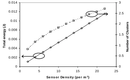
To see the impact of sensor density on the network energy consumption, we fixed the CH probability based on Popt obtained using (11). The total energy usage for
different sensor density (λ) is depicted in Fig. 2. It is evident that the total energy dissipated is linearly related to the density. However, these energy values are rather optimistic as we assume the wireless channel is error-free. When the node density is increased, there are more nodes in the same region resulting in higher total energy usage. With more nodes in the network, the second curve in Fig. 2 indicates that the number of clusters also increases albeit very marginally. This observation is consistent with the Popt curve depicted in Fig. 3. It is
evident that as the node density is increased, the optimal Popt reduces implying the formation of larger clusters
expending more energy.
0 0.002 0.004 0.006 0.008 0.01 0.012 0.014
0 5 10 15 20 25 Se ns or De ns ity (pe r m2)
T
o
tal
en
erg
y
(
J
)
0 0.5 1 1.5 2 2.5 3
Nu
m
b
er
o
f
Clu
s
te
rs
0 0.0005 0.001 0.0015 0.002 0.0025 0.003 0.0035 0.004 0.0045
0 5 10 15 20 25
Se ns or De ns ity (pe r m2)
O
p
tim
a
l C
H
Pr
o
b
a
b
ili
ty
,
P
opt
Popt vs. sensor density.
Figure 3.
To see the impact of sensor density on the network lifetime, it is assumed that each sensor node is initially equipped with 20 J energy, and there is a single transmission in every round of 20 seconds. As shown in Fig. 4, the node density has a logarithmic effect on network lifetime. Initial increase of the density significantly improved the network lifetime, as more nodes are available in the network to share the energy intensive operation of a CH function. However, any further increase only has marginal effect. This is mainly due to the presence of more members per cluster, which increases the average energy consumption per cluster. Thus, any further introduction of nodes into the network has a decreasing rate of improvement on the network lifetime. This implies that to deploy nodes in a region, there is a trade-off between the monitoring fidelity and network lifetime expectancy even when the optimal number of clusters is formed.
874 875 876 877 878 879 880 881
0 5 10 15 20 25
Se ns or De ns ity (pe r m2)
N
e
tw
o
rk
L
if
e
ti
m
e
(da
y
s
)
Figure 4. Lifetime vs. sensor density for A = 100 m2.
To see the impact of the CH probability against network lifetime for different number of nodes, the same setting as above is used. From Fig. 5, it is observed that there is an optimal CH probability that assures maximal network lifetime. It is found that this optimal value corresponds to the Popt value obtained using eqn. (11) and
is consistent with the total energy usage plot of Fig. 1. Thus, based on a specific scenario, we can ensure its optimal operation when the CH probability is configured using its Popt value. It can also be observed in Fig. 4 that
the increase of number of nodes has smaller improvement in the lifetime especially at higher level (c.f. 1500-2000 with 2000-2500 nodes), consistent with the result reported in Fig. 4.
876.5 877 877.5 878 878.5 879 879.5 880 880.5 881
0 0.001 0.002 0.003 0.004 0.005 0.006 0.007 0.008 CH Probability
Ne
tw
o
rk
L
ife
ti
m
e
(d
a
y
s
)
n = 1500 n = 2000 n = 2500
Figure 5. Network lifetime vs. CH probability
for n = 1500, 2000 and 2500.
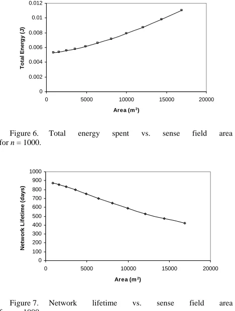
To investigate the effect of terrain size for a given number of sensor nodes, we assumed that n is 1000 nodes. As expected, Fig. 6 depicts an increase in total energy spent for increasing field area. As the area becomes larger, the node density reduces for a fixed number of nodes. Furthermore, the distance between nodes also increases. Thus, the total energy spent grows significantly. Consistent result is also obtained for the network lifetime as shown in Fig. 7. As more energy is dissipated per round, the overall network lifetime becomes shortened for larger fields.
0 0.002 0.004 0.006 0.008 0.01 0.012
0 5000 10000 15000 20000 Area (m2)
To
ta
l E
ne
rgy
(
J
)
Figure 6. Total energy spent vs. sense field area
for n = 1000.
0 100 200 300 400 500 600 700 800 900 1000
0 5000 10000 15000 20000 Area (m2)
N
e
tw
or
k
L
ife
ti
m
e
(da
y
s
)
Figure 7. Network lifetime vs. sense field area
From these results, it is obvious that we are able to accurately quantify the total energy usage as well as network lifetime for various network parameters such as number of clusters, sensor density and network area. The analytical equations derived based upon a realistic radio energy dissipation model allow us to determine the optimal CH probability and the corresponding minimal energy level readily. As the number of nodes to be deployed and the chosen region size are within one’s control, the optimal CH probability could be directly configured into the nodes prior to deployment.
V. CONCLUSION AND FUTURE WORK
As energy-awareness is highly critical in the design of sensor networks, we proposed the Time-Controlled Clustering Algorithm (TCCA) that does not require location information a priori. The objective of TCCA is to minimize the total energy dissipated by using non-monitored rotating clusterhead election. TCCA is also able to control a cluster’s diameter based on the message TTL and approximate its nodes’ distance to clusterheads using the message timestamp, which could be used to create a collision-free transmission schedule. An analytical model of this algorithm is derived based on the results from stochastic geometry to determine a realistic energy dissipation and network lifetime patterns. It was demonstrated that there is an optimal probability, which could easily be determined from the given expression and pre-configured into the nodes, to achieve an overall energy efficient operation. It was also found that there is a decreasing improvement on network lifetime, when more nodes are deployed within the same region.
As part of our current research we have assumed that the environment was collision and error free. The integrated use of the message timestamp and a suitable MAC protocol for the creation of collision-free transmission schedule is left for future work. Also, the current TCCA proposal does not ensure a uniform distribution of the elected CHs resulting in sub-optimal network operation. Achieving a uniform CH distribution would result in more equitable cluster sizes as well as the complete coverage of the nodes. Moreover, a more deterministic CH election approach might be useful that elects the optimal number of CHs (as per the given equation) throughout the network operation.
ACKNOWLEDGMENT
This work was supported in part by grants from ARC Discovery Project DP0664782 and USyd R&D L2844 U3230.
REFERENCES
[1] I. F. Akyildiz, W. Su, Y. Sankarasubramaniam and E. Cayirci, “Wireless sensor networks: a survey,” Elsevier
Journal of Computer Networks Vol. 38 No. 4, 2002, pp.
393–422.
[2] E. Shih, S. Cho, N. Ickes, R. Min, A. Sinha, A. Wang and A. Chandrakasan, “Physical layer driven protocol and algorithm design for energy-efficient wireless sensor
networks,” Proceedings of ACM MobiCom’01, July 2001, pp. 272–286.
[3] B. Warneke, M. Last, B. Liebowitz and K.S.J. Pister, “Smart Dust: Communicating with a Cubic-Millimeter Computer,” IEEE Computer Magazine Vol. 34 No. 1, Jan. 2001, pp. 44- 51.
[4] G. J. Pottie and W. J. Kaiser, “Wireless Integrated Network Nodes”, Communications of the ACM, Vol. 43, No. 5, May 2000, pp 51-58.
[5] J. M. Kahn, R. H. Katz and K. S. J. Pister, “Next Century Challenges: Mobile Networking for Smart Dust,” Proc. of
5th Annual ACM/IEEE International Conference on
Mobile Computing and Networking, Aug. 1999, pp.
271-278.
[6] D. J. Baker and A. Ephremides, “The Architectural Organization of a Mobile Radio Network via a Distributed Algorithm, IEEE Trans. on Comm. 29(11) (Nov. 1981) 1694-1701.
[7] B. Das and V. Bharghavan, “Routing in Ad-Hoc Networks Using Minimum Connected Dominating Sets,”
Proc. of ICC, 1997.
[8] C. F. Chiasserini, I. Chlamtac, P. Monti and A. Nucci, “Energy Efficient design of Wireless Ad Hoc Networks,”
Proceedings of European Wireless, February 2002.
[9] W. Heinzelman, A. Chandrakasan and H. Balakrishnan, “Energy-Efficient Communication Protocol for Wireless Microsensor Networks,” Proc. of IEEE Proc. Of the
Hawaii International Conf. on System Sciences, Jan.
2000, pp. 1-10.
[10] M. J. Handy, M. Haase and D. Timmermann, “Low energy adaptive clustering hierarchy with deterministic cluster-head selection,” Proc. of IEEE Int. Conf. on
Mobile and Wireless Comm. Networks, Sept. 2002, pp.
368 – 372.
[11] S. Bandyopadhyay and E. J. Coyle. An energy efficient hierarchical clustering algorithm for wireless sensor networks. Proc. of the 22nd Joint Conf. of the IEEE
Computer and Comm. Societies, June 2003, pp.
1713-1723.
[12] S. Selvakennedy and S. Sinnappan, “The Time-Controlled Clustering Algorithm for Optimized Data Dissemination in Wireless Sensor Networks,” Proc. Of IEEE Conference
on Local Computer Networks, Sydney, Australia, Nov.
2005, pp. 509-510.
[13] A. Perrig, R. Szewczyk, V. Wen and J. D. Tygar, “SPINS: Security protocols for Sensor Networks,” Proc. 7th Annual Int. Conf. on Mobile computing and Networking
(2001) 189-199.
[14] D. W. Carman, P. S. Kruus and B. J. Matt, “Constraints and approaches for distributed sensor network security,”
NAI Labs Technical Report 00-010, Sept. 2000.
[15] N. Bulusu, J. Heidemann and D. Estrin, “Adaptive beacon Placement,” Proc. of the Twenty First Int. Conference on
Distributed Computing Systems (ICDCS-21), April 2001.
[16] A.D. Amis and R. Prakash, “Load-Balancing Clusters in Wireless Ad Hoc Networks,” Proc. of ASSET 2000, March 2000.
[17] A. Ephremides, J.E. Wieselthier and D. J. Baker, “A Design concept for Reliable Mobile Radio Networks with Frequency Hopping Signaling, IEEE Vol. 75 No. 1, 1987, pp. 56-73.
[18] C. R. Lin and M. Gerla, “Adaptive clustering for mobile wireless networks,” J. Select. Areas in Comm. Vol. 15, Sept. 1997, pp. 1265-1275,.
Architectures, Algorithms and Networks (I-SPAN ’99), June1999, pp. 310-315.
[20] M. Chatterjee, S.K. Das and D. Turgut, “WCA: A Weighted Clustering Algorithm for Mobile Ad hoc Networks,” Kluwer Journal of Cluster Computing,
Special issue on Mobile Ad hoc Networking, Vol. 5, 2002,
pp. 193-204.
[21] S. Ghiasi, A. Srivastava, X. Yang, and M. Sarrafzadeh, “Optimal Energy Aware Clustering in Sensor Networks,”
Nodes Magazine MDPI 1, Jan. 2002, pp. 258-269.
[22] A. D. Amis, R. Prakash, T. H. P. Vuong and D. T. Huynh, “Max-Min D-cluster formation in wireless ad hoc networks,” Proc. of IEEE INFOCOM, Mar. 2000.
[23] S. G. Foss and S.A. Zuyev, “On a Voronoi Aggregative Process Related to a Bivariate Poisson Process,”
Advances in Applied Probability Vol. 28 No. 4, 1996, pp.
965-981.
[24] B. J. Culpepper, L. Dung and M Moh, “Design and analysis of Hybrid Indirect Transmissions (HIT) for data gathering in wireless micro sensor networks,”
SIGMOBILE Mobile Computing Comm. Review Vol. 8
No. 1, 2004, pp. 61-83.
[25] S. Lindsey, C. Raghavendra and K. Sivalin, “Data Gathering Algorithms in Sensor Networks Using Energy Metrics,” IEEE Trans. on Parallel and Dist. Systems, Sept. 2002, pp. 924-935.
[26] W. Ye, J. Heidemann and D. Estrin. “An energy-efficient MAC protocol for wireless sensor networks,” Proc. of
21st Conf. of the IEEE Comp. and Comm. Soc., June
2002, pp. 1567-1576.
S. Selvakennedy obtained his PhD in computer
communications in 1999 from the University of Putra, Malaysia. Earlier in 1996, he obtained his first-class honors degree in computer science also from the same university.
He is currently serving as a Senior Lecturer at the University of Sydney, Australia. He has published more than 50 articles in journals and conferences mainly in the area of communications protocols for all-optical networking and wireless networking. His current research interests lies in developing algorithms for media access, routing, localization and topology control issues in wireless sensor networks, wireless ad hoc networks and wireless mesh networks. Dr. Selvakennedy is a member of ACM and IEEE.