Application of Spatial Regression Models to Income Poverty Ratios in Middle Delta Contiguous Counties in Egypt

in Middle Delta Contiguous Counties in Egypt

Sohair F Higazi Dept. Applied Statistics

Faculty of Commerce, Tanta University, Tanta, Egypt [email protected]

Dina H. Abdel-Hady Dept. of Statistics Faculty of Commerce

Tanta University, Tanta, Egypt [email protected]

Samir Ahmed Al-Oulfi Faculty of Commerce Mansoura University, Egypt [email protected]

Abstract

Regression analysis depends on several assumptions that have to be satisfied. A major assumption that is never satisfied when variables are from contiguous observations is the independence of error terms. Spatial analysis treated the violation of that assumption by two derived models that put contiguity of observations into consideration. Data used are from Egypt's 2006 latest census, for 93 counties in middle delta seven adjacent Governorates. The dependent variable used is the percent of individuals classified as poor (those who make less than 1$ daily). Predictors are some demographic indicators. Explanatory Spatial Data Analysis (ESDA) is performed to examine the existence of spatial clustering and spatial autocorrelation between neighboring counties. The ESDA revealed spatial clusters and spatial correlation between locations. Three statistical models are applied to the data, the Ordinary Least Square regression model (OLS), the Spatial Error Model (SEM) and the Spatial Lag Model (SLM).The Likelihood Ratio test and some information criterions are used to compare SLM and SEM to OLS. The SEM model proved to be better than the SLM model. Recommendations are drawn regarding the two spatial models used.

Keywords:Spatial Regression, Spatial Error Model, Special Lag Model, GeoDa, ESDA, LISA Maps.

Introduction

Spatial data is data collected from contiguous units. It has been introduced in 1988 by Luce Anselin, and was first applied in some econometric model, and then followed by several studies to name a few, in criminology, environmental studies, epidemiology, regional economics (Haining 2003), immigration and demographic studies (Voss 2007, Haining 2003), real estate (Pace and Barry 1998, Haining 2003), poverty studies (Voss 2006, Friedman and Lichter 1998), child povertyi_{and in agricultural economics (Lambert}

Several spatial data analysis packages, such as MATLAB (Lesage 1998), SpacStat (Anselin 1992), GeoDaii _{contribute to a great extent in the spreading of spatial data}

analysis. Spatial data could be cross sectional or data collected over a short period of time that is believed that time does not affect the measurements taken. Spatial data differs than time series data since the later puts the "time" rather than the "site" into consideration. Spatial data analysis depends on "organizing" data in "neighboring" clusters, these neighbors are homogeneous "within" and heterogeneous "between" with respect to some variables. Thus, the assumptions of ordinary least squares regression are violated, especially, the assumptions of homogeneity and of independence of error terms.

Spatial analyses differ than spatial data analysis, while the former depends mainly on GISiii _{tools to discover relationships and similarities between units studied, the later uses}

statistical data analysis tools and Exploratory Spatial Data Analysis (ESDA) to discover spatial statistical relationships between contiguous units; for example, studying the spatial relationship between the occurrence of Leukemia among children who live close to high voltage power cables, or the spatial relationship between Alzheimer and water source with high aluminum deposits in some areas. However, Geo-statistical methods provide a set of spatial statistical methods for describing and analyzing the patterns of spatially distributed phenomenon (Anselin 1995 2006).

The present study presents how to discover spatial correlation, and how to measure it using ESDA. The study introduces and applies two spatial regression models to predict percentage of persons under poverty line in 93 counties in seven neighboring governorates in lower Egypt, using some demographic indicators as explanatory variable (CAPMAS 2006), in an attempt to find out do neighboring counties share the same demographic characteristics? Can we reach a different prediction equation for neighboring counties?

In Section 1, spatial data analysis concepts are introduced; in Section 2, we present spatial regression models; in Section 3, the spatial statistical data analysis results are shown; conclusions and recommendations are given in Section 4,

1. Spatial Data Analysis

Spatial data is characterized by having "location" or "Spatial" effects, where there are Spatial heterogeneity between and spatial homogeneity within neighboring clusters; thus "spatial dependence" is exhibited among these clusters. When these characteristics are ignored using Ordinary Least Squares (OLS) in linear regression analysis, for example, the resulting parameter estimates are biased, inconsistent and the R2 _{values is not an}

accurate fitness of fit measure, since the assumption of independent error terms is violated since spatial dependence and spatial autocorrelation exist in the data.

    otherwise 0 j neighbor i 1 W

not equal zero, and no autocorrelation exists otherwise (Haining 2003). One of the most spatial autocorrelation measures is Global Moran's I measure which depends on a "weight matrix". A wide range of criteria may be used to define neighbors, such as "binary" contiguity (common boundary) or "distance" bands (Getis, and Ord 1995) or "queen" contiguity, meaning that the neighbors for any given location 'A' are all other locations share a common boundary with 'A' in any direction. In general, the weight matrix takes the value "0" or "1" as follows:

For example, the weight matrix for the shown neighboring units (Haining 2003 p. 83) is:

Thus;

The weight matrix is then normalized such that:

ij i ij ij _w w w 

 0 wij≤1 (1)

Tests for spatial autocorrelation for a single variable in a cross-sectional data set are based on the magnitude of an indicator that combines the value observed at each location with the average value at neighboring locations (called spatial lags). Basically, the spatial autocorrelation tests are measures of the similarity between association in values (covariance, correlation or difference) and association in space (contiguity). Spatial autocorrelation is considered to significant when the spatial autocorrelation statistic takes on an extreme value, compared to what would be expected under the null hypothesis of no spatial autocorrelation (Anselin 1992).

To measure Spatial Autocorrelation, Global Moran I coefficientiv _{is used, it takes the} form:







j ij i j n

i n

j ij y y

y y y y w w n I 1 2 1 1

1 1 ( )

) )(

(

(2)

Where wijisas defined in [1] above. Moran I is interpreted as Pearson's Product moment

correlation coefficient. The spatial autocorrelation for neighboring units is called Local Moran I, it takes the weights of unit i and unit j within the same cluster into consideration as follows:

 



When significant spatial autocorrelation, (spatial dependence) exists either globally or locally, spatial heterogeneity exists (Anselin 1988, Lesage 1998) and accordingly non-constant errors. There are several diagnostic tests that could be used to test the significance of spatial effects, such as examining residuals from OLS to reveal heterogeneity of variances. However, this requires special software programs that depend on maps to determine the "locations" of units. Spatial effects are tested using Breusch Pagan test (Breusch and Pagan 1979 ) for testing homogeneity assumption, Moran test , Lagrange Multiplier (LM) lag test and LM-error tests for testing spatial autocorrelation (Haining,2003). Also, ESDA results such as residual plots and residual maps are examined to locate extreme values and reveal heterogeneity, globally and locally.

2. Modeling Spatial Regression

Spatial regression models are used as a next step to ESDA. When ESDA reveals Local

Indicator for Spatial Autocorrelation, LISA, (Anselin 1994 1998 1999a, Haining 2003, Bailey and Gatrell 1995). Haining (2003) has introduced two spatial regression models: the "SpatialLagModel (SLM)" and the "SpatialErrorModel (SEM)".

The Ordinary Least Squares regression model takes the form:

) ( ) ( ) ( 2 2 ) ( 1 1 0 )

(i x i x i .... kxk i ei

y       i1...,n (4)

Where y(i) is normally distributes, n is the number of units studied, and e(i) are i.i.d.

) , 0 ( _2

N .

(Voss et al , 2006).When spatial autocorrelation exists, in [4] above, the error term has to take this autocorrelation into account as follows:

) ( ) ( ) ( 2 2 ) ( 1 1 0 )

(i x i x i ... kxk i ui

y       i1...,n (5)

Where, u(i) is the spatially correlated error term, it is distributed as multivariate term:

T

n u u

u( (1),... ( )) uMVN(0,V)

The spatial effects fall within the matrix V, arising from the contiguity structure via the weight matrix as follows (Haining, 2003):

) ( ) ( (, ) ( ) ) ( ) ( 2 2 ) ( 1 1 0 )

(i x i x i ... kxk i _{j N i} wi j y j ei

y      



(6)

n i1...,

Where ρ is a spatial effect parameter, w(i,j) is the normalized weight matrix as in [1]

above,N(i) are the number of contiguous units for unit i, and the term



N(i) ( , ) ( )

j w i j y j

 expresses how the regression equation is affected by the spatial effects.

Two models stem from [6] above, namely theSpatialErrorModel (SEM) and theSpatial

LagModel (SLM). TheSEMtakes the form:

i j

ij

j ij j

i

x

w

y

y



















Where,  is the spatial error lag coefficient, and iarei.i.d, in matrix form, Equation (7)

is written as:

(8)

The matrix WY is used as an additive explanatory variable, calculated by using the spatially lagged dependent variable according to the weight matrix. The predicted value is:(_{I }ˆ_W)1_Xˆ_{, the model residual error is (IˆW)yX}ˆ _{and the prediction error}

is:(Y Y).

The SLM takes the form

i j

j ij

j

j ij

i

x

w

u

y

















In matrix form:

u

W

X

Y













Where,



error for location i. The predicted value is: (_{I }_W)1_Xˆ_{, the model residual error is} 

 ) ˆ

(I W yX and the prediction error is:(Y Y). i

WY

X

The variance-Covariance matrix of



1 1

2

(

)

(

)

)

(













e

e



I



W

I



W

The maximum likelihood (ML) estimation procedure is used for the estimation of the parameters of both the SEM and the SLM (Upton et al 1985). The ML function for the SLM (Haining 1990) is:

] ) )( ) ( ( ) ( [ 2 1 ln ln 2 2 ln 2 ) , , ( 1 2 2 2 y W I X X X X I W I y W I N N                        

And for the SEM is:

)] )( ( ) ( ) [( 2 1 ln ln 2 2 ln 2 ) , , ( 2 2 2            X y W I W I X y W I N N             

And thus the two models may be compared to the OLS model, and the following parameter may be tested, H0:0 againstH1:0 for SLM, and for SEM, we test

0 : against 0

: 1

0   H  

H ; testing is performed by Wald test, Likelihood Ratio

test and Lagrange Multiplier (LM) test Anselin 1988b).

3. Application Results

Poverty is a reflection of many economic and living conditions (unemployment, illiteracy rate, average GDP, education drop-outs, access to sanitation facilities, dependency ratios, health care . . . etc). Income poverty is measured in this paper as the proportion of the population with a level of income below one dollar per day (166 Egyptian pounds monthly). Nation wide, this percentage is 19% (CAPMAS 2006).

The variability in spatial distribution of poverty is related to its geographic determinants such as differences in geographic conditions. A poverty map increases the visibility and perceptibility in spatial heterogeneity of poverty at a higher disaggregated level. However, it does not provide an estimate of the relationship between spatial patterns of poverty and spatial variables that influence it (Petrucci, et al, 2003).

The main objective of the study is to investigate the relationship between selected spatial variables and the level of poverty in middle Delta counties in Egypt.

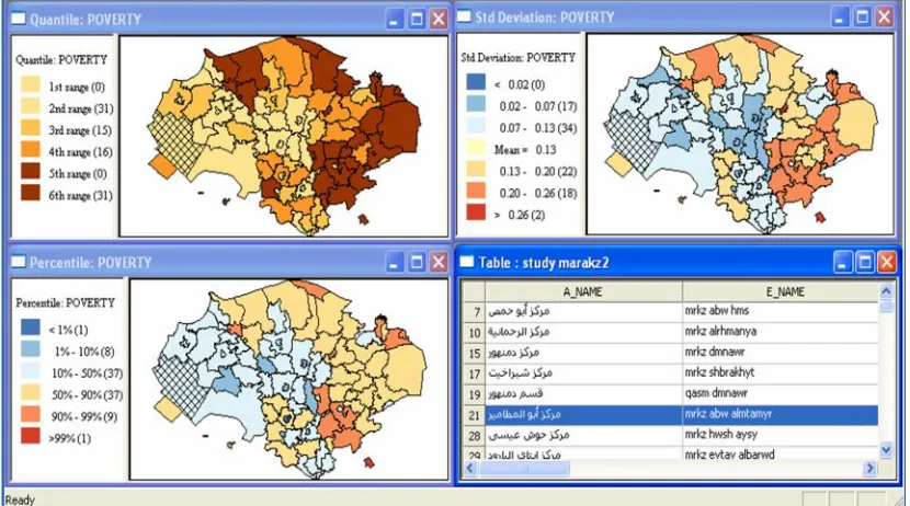
The study includes 93 contiguous counties in seven governorates, the spatial statistical package "GeoDa" is used, it depends on a digital map, ArcGis 9.2 GIS is used to input spatial data (data file is called Markaz, means "county"); clicking on any county in the data file shows its location on the map (Map 1).

The dependent variable used is the proportion of persons under poverty line. A preliminary ESDA is performed to reveal statistically non-significant explanatory variable; the "average family size" (r = 0.05), "percentage of higher than secondary school holders", (r= -0.06) were non-significant and were excluded from the analysis. Thus, explanatory variables used are: illiteracy rate (il_lit), dependency ratio (dep_r), percent of education drop outs (ed_drop), unemployment rates un_emp) and percent of (temporary workers (temp_w). Table [1] gives some descriptive measures on variables used in the study (n=93).

OLS model is applied using the significant explanatory variables (α=5%), the model proved significant (R2_{= 0.17, P <0.01).}

An ESDA descriptive measure for the response variable (poverty ratio) is performed. Some explanatory data analysis maps are obtained, (spatial clusters [Map 2] are evident from these maps). The mean poverty ratio is 13%, 51 counties are below the mean, 22 counties between 13 to 20%, and 20 counties are above 20%. When clicking on any county in the Table high lightened on Map2, and clicking on any county on the map, is high lightened on the table (Quadrant 4).

Map 2: ESDA for Poverty Ratios Table 1: Descriptive Measures

93 .02167 .30000 .1347568 .06180393 93 .011 .085 .03551 .017040 93 .104 .500 .29641 .078283 93 .022 .173 .09176 .032316 93 .491 .694 .58552 .042476 93 .103 .909 .27832 .120760 93

Variable poverty ed_drop il_lit un_emp dep_r temp_w Valid N (listwise)

Global Moran I

A fundamental concept in the analysis of spatial autocorrelation for areal data is the spatial weights matrix. In this paper a spatial weights matrix of the queen first order was used to formalize a notion of location.

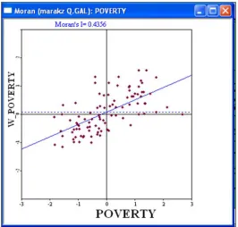
In the Moran scatter plot of poverty ratios are exhibited in Figure 1. Data are standardized so that units on the graph are expressed in standard deviations from the mean. The horizontal axis shows the standardized value of "poverty" for a county, the vertical axis shows the standardized value of the average poverty rates (Spatial Lag Poverty (W-Poverty)), for that county’s neighbors as defined by the weights matrix.

Figure 1: Global Moran Scatter Plot, SEM

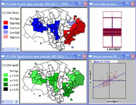
The Univariate Local Indicators of Spatial Autocorrelation "LISA" (Anselin, 1995 2003) shows significant autocorrelation (shown as colored clusters on Map 3, given to the right).

Thus, the diagnostics tests for spatial dependence showed the presence of spatial autocorrelation. Table (2) gives Global Moran autocorrelation coefficients between poverty levels and each explanatory variable. All Moran's coefficients are significant (P<0.001).

Table 2: GeoDa Global Moran I for each explanatory Variable Explanatory Variable Moran I

Education Drop-out ratio 0.3421

Illiteracy Rate 0.2514

Unemployment rate 0.139

Dependency Ratio 0.3924

Temporary Workers ratio 0.3492

Spatial Regression Models

A classical regression was performed first to model the functional relationship between county level poverty and selected spatial variables. Three different analyses were performed: First, Ordinary Least Squares (OLS) regression is performed as a reference model; secondly, estimation by means of maximum likelihood of a spatial regression model that includes a spatially lagged dependent variable, and thirdly, estimation by means of maximum likelihood of a spatial regression model that includes a spatially lagged error.

a. Ordinary Least Square Regression

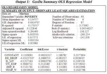
Explanatory variables used were: illiteracy, unemployment, education drop-outs, and dependency and temporary workers rates. OLS summary output is given in output (1) below, the only significant variable (α=5%) was: "dependency Ratio. The produced R2 value is 17% (P<0.01), the OLS F- statistic is significant (P<.01).

Output 1: GeoDa Summary OLS Regression Model

Thus, the following reference criterions are obtained:

Table 3: OLS Information Criterion

136.127 Log likelihood

-260.254 Akaike info criterion

-245.058 Schwarz criterion

Diagnostic tests for OLS assumptions ( Output 2) showed that multi-co linearity is of no problem according to the conditional number of Belesley et al (1980), Jarque-Bera test reveals that error are not normally distributed, Breusch-Pagan, White and Koenker-Bassette tests (Haining 2003) reveal heterogeneity of error variance.

Output 2: GeoDa OLS Regression Diagnostic Tests

Output 3: GeoDa Diagnostic Tests for Spatial Dependence

The Quantile OLS Predicted Map (Map 4) gives the variations not included in the error term; it is evident that there are clusters of the same color. Also, the OLS Residual map (Map 5) shows the existence of spatial autocorrelation between poverty ratio and the set of explanatory variables used. Thus, spatial regression models are recommended.

Map 4: OLS_ Predict Quantile Map

Map 5: OLS Residual Map b. Spatial Error Model (SEM)

GeoDa output for SEM is shown in output (4). The obtained R2 _{value is 43.44%, the lag}

Output 4: GeoDa Summary of Spatial Error Regression Model

Table 4: Information Criterion for OLS and SEM

Model OLS SEM

Log likelihood 136.127 149.33

AIC -260.254 -286.661

SC -245.058 -271.465

A limited number of diagnostics are provided with the ML Error estimation, as illustrated in Output (5). First is a Breusch-Pagan test for heteroskedasticity in the error terms. The insignificant value of 7.23 suggests that there is heteroskedasticity, as in the OLS. The second test is an alternative to the asymptotic significance test on the spatial autoregressive coefficient; the Likelihood Ratio Test is one of the three classic specification tests comparing the null model (the classic regression specification) to the alternative spatial lag model. The highly significant value of 26.5 (Output 5) confirms the strong significance of the spatial autoregressive coefficient. The other two classic tests are the Wald test, which is the square of the asymptotic t-value (or, z-value), and the LM-Error test based on OLS residuals.

According to Anselin (2005), in finite samples, the W  LR  LM should hold true; Checking the order of the W, LR and LM statistics on the spatial autoregressive error coefficient, the Wald test (Output 4) is W= (8.383)2 _{= 70.3 LR=26.40 (output 5)}

Output 5: GeoDa Spatial Error Model Diagnostics

Figure 3, gives Moran I scatter plot for SEM. In Figure 3, ERR RESIDU contains the model residuals (ˆu), ERR PREDIC the predicted values (ˆy), and ERR PRDERR the prediction error (y − ˆy). To construct a Moran scatter plot for both residuals, ERR RESIDU and ERR PRDERR Residuals. A Moran I=0.0085 reflects very weak correlation, which means including the spatial autoregressive error term has eliminated all spatial effects from the model. Moran I for ERR PRDERR and the model residuals (W_ERR RESID), I= 0.4892 is very close to Moran I obtained from OLS; the scatter plot obtained reflects linear relationship between error prediction error( ERR PRDERR) and the error predicted values (W_ERR RESUD) according to SEM, it is an estimate of the spatially produced error terms.

Figure 3: Moran scatter plot for Spatial Error Model Residuals

The SEM model is estimated as



i i

W

W

temp

R

dep

emp

un

lit

il

drop

ed

y

*

701

.

0

_

*

075

.

0

_

*

240

.

0

_

*

403

.

0

_

*

006

.

0

_

*

38

.

0

16

.

0

ˆ















c. Spatial Regression Lag Model (SLM)

Called also Spatial Auto-Regressive Model(SAR). The model takes the form:

)

,

0

(

,

X

Wy

Y

















N



I

Where; Wyis a lagged poverty ratios, it is the average of all poverty ratios in all contiguous counties, according to the weight matrix used. This model evaluates the strength of spatial relationship between poverty ratios in all contiguous counties. The following output is obtained:

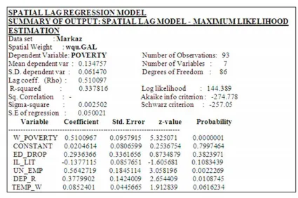
Output 6: GeoDa Summary of Spatial Lag Regression Model

The obtained R2value is 33.78%, the lag coefficient ρ= 0.51 is significant ( P<.01), the information criterion obtained are compared to those obtained from OLS ( Table 3 and Table 4) and SEM, as shown in Table 6, where it is evident that both SEM and SLM are better than OLS, but the SEM is better than the SLM.

Table 6: Information Criterion for OLS, SEM and SLM

Model OLS SEM SLM

Log likelihood 136.127 149.33 144.38

AIC -260.254 -286.661 -274.778

The estimated SLM modelis:

i y i

W

*

51

.

0

W

_

temp

*

085

.

0

R

_

dep

*

378

.

0

emp

_

un

*

564

.

0

lit

_

il

*

114

.

0

drop

_

ed

*

293

.

0

02

.

0

yˆ















Where, Wyi is the average Poverty ratios in all neighboring counties, according to the weight matrix used. The SLM diagnostic tests (Output 7) shows heterogeneity of the error term (Breusch-pagan test is significant). The likelihood ratio test for the comparison of the SLM model to the OLS model is:

   

  

OLS spatial

L L Log 2

LR = 16.25 (P<0.01).

Anselin (2005), ordering of W  LR  LM _{is satisfied.}

Output 7: GeoDa Spatial Lag Regression Diagnostic Tests

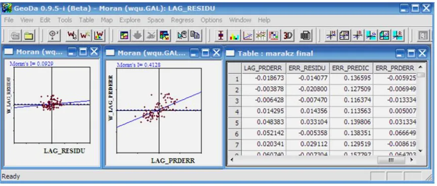
Figure 4, gives Moran I scatter plot. In Figure 4, LAG RESIDU contains the model residuals (ˆu), LAG PREDIC the predicted values (ˆy), and LAG PRDERR the prediction error (y − ˆy). Residuals and prediction error could be used as an examination tool for the spatial SLM. A Moran I=0.0929 reflects very weak correlation, which means including the spatial autoregressive lag term has eliminated all spatial effects from the model. Moran I for LAG- PRDERR and W_LAG RESID (I= 0.4126) is very close to Moran I obtained from OLS; the scatter plot obtained reflects linear relationship, between lag prediction error and the lag predicted values according to SLM.

4. Conclusions

The main objective of the study is to apply spatial regression models to contiguous data. Data used are from the 2006 latest census, for all 93 counties in middle delta adjacent Governorates. The dependent variable used is the percent of individuals classified as poor (those who make less than 1$ daily). Predictors or explanatory variables used are the ratios of illiteracy, dependency, temporary work, education drop-out, and unemployment. The spatial analyses depend mainly on the geographic map of all counties under study. Maps and data are obtained from CAPMAS (Central Agency for Public Mobilization and Statistics).The researcher input the map using .shape file, and data and map are analyzed using a spatial analysis package " GeoDa".A Spatial Explanatory Data Analysis (SEDA) is performed to each variable of the variables under study, to examine the existence of spatial clustering and spatial correlation between neighboring counties. The SEDA revealed spatial clusters and spatial correlation between locations.

Three statistical models are applied to the data. The Ordinary Least Square regression model (OLS). The assumptions of OLS model are tested, and the OLS shows a very low R2_{value and not all its assumptions were satisfied, especially the independence of the}

error term and the homogeneity of variance assumption.

Spatial Regression analysis models depend mainly on a "Weight Matrix". For the data under study ( 93 counties) a matrix (93x93) with elements either "0" or "1" ; where "0" is

given when a county i is not a neighbor to county j (i≠ j), and "1" when county i is a neighbor to county j.

Two models are applied. The Spatial Error Model (SEM) introduces an extra variable to the predictors in the model. That added variable is the average of the error terms in the neighboring counties, using the weight matrix. The other model is the Spatial Lag Model (SLM) which introduces also an extra variable to the predictors in the model, that added variable, is the average of the dependent variable in the neighboring areas.

Diagnostic tests for independence of error terms, homogeneity of variance and normality are performed for each model. Spatial autocorrelation are also obtained.

A comparison between all results was made. The SEM model proved to be better than the SLM model as far as the value of R2 _{and with respect to the information criterion (ML,}

Akaike, Schwarz criterion). The Likelihood Ratio test is used to compare SLM and SEM to OLS. Recommendations are drawn regarding the two spatial models used, and recommendations are reached for decision makers with regard to the spatial dependence of all variables used in the analysis, and neighboring counties which need more attention and more allocation of resources in the area of education, family planning, employment are pinpointed.

References

1. Anselin, Luc. (1988). Spatial Econometrics, Methods and Models. Dordrecht: Kluwer Academic.

2. Anselin, Luc (1988a). "Model Validation in Spatial Econometrics: A Review and Evaluation of Alternative Approaches", International Regional Science Review

3. Anselin, Luc (1988b). "Lagrange Multiplier Test Diagnostics for Spatial Dependence and Spatial Heterogeneity", Geographical Analysis 20, 1-17.

4. Anselin, L. (1992), SpaceStat: A program for the analysis of spatial data. National Center for Geographic Information and Analysis, University of California, Santa Barbara.

5. Anselin, Luc (1994). “Exploratory Spatial Data Analysis and Geographic Information Systems.” PP. 45-54 in New Tools for Spatial Analysis, edited by M. Painho. Luxembourg: Euro-Stat.

6. Anselin, L. (1995). "Local Indicators of Spatial Association—LISA",

Geographical Analysis27:93-115.

7. Anselin, Luc (1996), “The Moran Scatter Plot as an ESDA Tool to Assess Local Instability in Spatial Association.” Pp. 111- 125 in Manfred Fischer, Henk J. Scholten and David Unwin (eds.) Spatial Analytical Perspectives on GIS. London: Taylor & Frances.

8. Anselin, Luc and Anil Bera. (1998). “Spatial Dependence in Linear Regression Models with an Introduction to Spatial Econometrics.” PP. 237-289 in Aman Ullah and David Giles (eds.) Handbook of Applied economic Statistics. New York: Marcel Dekker.

9. Anselin, L. (1999). "The Future of Spatial Analysis in the Social Sciences".

Geographic Information Sciences5(2): 67-76.

10. Anselin, Luc (1999a). “Interactive Techniques and Exploratory Spatial Data Analysis.” Pp. 251-264 in Geographic Information Systems: Principles, Techniques, Management and Applications, edited by P.A. Longley, M.F. Goodchild, D.J.

11. Anselin, Luc. (2003). An Introduction to Spatial Autocorrelation Analysis with GeoDa. Spatial Analysis Laboratory, University of Illinois. (http://sal agecon.uiuc.edu/csiss/pdf/spauto.pdf).

12. Anselin, Luc. (2003a). GeoDa 0.9 User’s Guide. Center for the Spatial Integration of social Sciences and Spatial Analysis Laboratory, University of Illinois. Urbana, IL: University of Illinois.(http://sal agecon.uiuc.edu/csiss/pdf/geoda093.pdf).

13. Anselin, Luc (2005). Exploring Spatial Data with GeoDaTM_{: A Workbook GeoDa}

0.9 User’s Guide. Center for the Spatial Integration of Social Sciences and Spatial Analysis Laboratory, Department of Geography ,University of Illinois, Urbana-Champaign, Urbana, IL 61801 http://sal uiuc.edu/ .

14. Anselin, L. (2006). Spatial Regression, National center for Supercomputing Applications, University of Illinois.

15. Armstrong, H.W. and Taylor, J. (2000). Regional Economics and Policy. New York: Harvester Wheat sheaf.

16. Bailey, N.T.J. (l967). "The Simulation of Stochastic Epidemic's in Two Dimensions". Proceedings. Fifth Berkeley Symposium on Mathematics and Statistics,4, 237-57. Berkeley and Los Angeles, CA: University of California. 17. Bailey, T.C. and A.C. Gatrell. (1995). "Interactive Spatial Data Analysis". New

York: John Wiley

19. Belsley, D., E. Kuh, R. Welsch (1980). "Regression Diagnostics, Identifying Influential Data and Sources of Collinearity Kluwer". New York: Wiley.

20. Breusch, T. and Pagan, A. (1979). A Simple Test of Heteroskedas-ticity and Rrandom Coefficient Variation.Econometrica47, 1287- 1294.

21. Central Agency for Public Mobilization Statistics (2006). 2006 Census, Cairo, Egypt.

22. Friedman, S. & Lichter, D.T. (1998). "Spatial Inequality and Poverty Among American children". Population Research and Policy Review91-109.

23. Ord, J.K. and A. Getis. (1995). "Local Spatial Autocorrelation Statistics: Distributional Issues and an Application". Geographical Analysis 27: 286-306. 24. Haining, R. P. (1990). "Spatial data analysis in the social and environmental

sciences”.Cambridge: Cambridge University Press.

25. Haining R. P. (2003). "Spatial Data Analysis, Theory and Practice", University of Cambridge Press.

26. Lambert, Dayton & Lowenberg-Deboer, Jess & Malzer, Gary (2005). "Managing Phosphorous Soil Dynamics Over Space and Time". 2005 Annual Meeting of the American Agricultural Economics Association, July 24-27, Providence, RI. 27. Lloyd, O.L. (1995). "The Exploration of the Possible Relationship between

Deaths, Births and Air Pollution in Scottish Towns: The Added Value of Geographical Information Systems",public Environmental Health.pp. 167-80. 28. Lesage, James P. (1998). "ECONOMETRICS: MATLAB tool box Components".

T961401, Boston College Department of Economics.

29. Ord, J.K. and A. Getis (1995). "Local Spatial Autocorrelation Statistics: Distributional Issues and an Application". Geographical Analysis 27: 286-306. 30. Otheringham, A.S. and Wegener, M. (2000). "Spatial Models and CIS".London:

Taylor & Francis.

31. Pace R.K., Barry, R. & Sirmans, C.F. (1998). "Spatial Statistics and Real Estate".

Journal of Real Estate Finance and Economics17(1): 5-13.

32. Petrucci, A., Nicola S., and Chiara S. (2003). "The application of a Spatial Regression Model to the Analysis and Mapping Poverty". FAO Natural Resources Service, No.7-ISSN 1684-8241. Retrieved August 9, 2008 from: http//fao.org/docrep/ 006/y4841 e00.htm.

33. Voss, Paul R., David D. Long, Roger B. Hammer, and Samantha Friedman. (2006)." County Child Poverty Rates in the U.S.: A Spatial Regression Approach". Population Research and Policy Review 25.

34. Voss, Paul R. (2007). "Demography as a Spatial Social Science". Population Research and Policy Review 26.

i_{https://www.geoda.uiuc.edu/Members/admin/pdf/county-child-poverty-rates-in-the-u-s.pdf.}

ii_{https://www.geoda.uiuc.edu/Members/admin/pdf/county-child-poverty-rates-in-the-u-s.pdf.} iii_{http://www.geostatistics.com/.}