on Industrial Networks and Intelligent Systems
Research Article
1
A Simulation Analysis of the Connectivity of Multi-hop
Path between Two Arbitrary Nodes in Cognitive Radio
Ad Hoc Networks
Le The Dung
1,*, Ba Cao Nguyen
2and Tran Manh Hoang
21
Department of Radio and Communication Engineering, Chungbuk National University, Republic of Korea 2
Faculty of Radio Electronics, Le Quy Don Technical University, Viet Nam
Abstract
The connectivity of multi-hop path is one of the key factors that influence the performance of multi-hop wireless networks. In this paper, assuming that secondary users (SUs) and primary users (PUs), using same licensed frequency bands, are uniformly distributed in square network area, we investigate the connectivity of multi-hop path in cognitive radio ad-hoc networks (CRAHNs). Specifically, we propose an algorithm to find all available multi-hop paths between arbitrary source node and destination node in CRAHNs with random node distribution and PU activity. Then, we use statistical simulation method to intensively evaluate the connectivity of multi-hop path compared with that in conventional ad-hoc networks (AHNs) by using huge number of random network topologies with different network parameters such as the number of SUs and PUs, network size, network operating frequency, and the average active rates of PU. The simulation results reveal many interesting and distinguishing features of the connectivity of multi-hop path in CRAHNs. Moreover, from the simulation graphs in this paper, network designers can select optimal network parameters so that the reliability of network topology is high while saving network resources. Finally, the simulation results can be used to verify mathematical models of the connectivity of multi-hop path in CRAHNs in future research.
Keywords: wireless ad-hoc networks, cognitive radio networks, multi-hop path, connectivity, statistical simulation method.
Received on 19 September 2019, accepted on 18 October 2019, published on 24 October 2019
Copyright © 2019Le The Dung et al., licensed to EAI. This is an open access article distributed under the terms of the Creative Commons Attribution licence (http://creativecommons.org/licenses/by/3.0/), which permits unlimited use, distribution and reproduction in any medium so long as the original work is properly cited.
doi: 10.4108/eai.24-10-2019.160984
*Corresponding author. [email protected]
1. Introduction
In recent years, technological advances together with the demand for efficient and flexible networks have led to the development of wireless ad-hoc networks. In such networks, mobile devices can communicate with each other in a peer-to-peer fashion with no need of for any base station or pre-existing network infrastructure. Ad-hoc networks have been mostly limited their operations in the 900 MHz and the 2.4 GHz industrial, scientific, and medical (ISM) bands. With the fast increase in the number of wireless devices, these frequency bands are getting congested. At the same time, many other licensed frequency bands allocated through static polices are used only in bounded geographical area or over specific period
of time. The Federal Communication Commission (FCC) estimated that the average utilization of licensed frequency band varies between 15-18% [1]. To address the critical problem of spectrum scarcity, FCC has recently approved the use of unlicensed devices in licensed bands. This policy has encouraged the development of Cognitive Radio Ad-Hoc Networks (CRAHNs) [2, 3] to improve spectrum usage efficiency. CRAHNs are distributed networks where unlicensed users (or Secondary Users – SUs) can coexist within the networks with licensed users (or Primary Users – PUs) if unlicensed users use licensed frequency bands opportunistically in a dynamic and non-interfering manner.
Many routing protocols have been proposed for disaster relief networks [4] and sensor networks [5, 6].
2
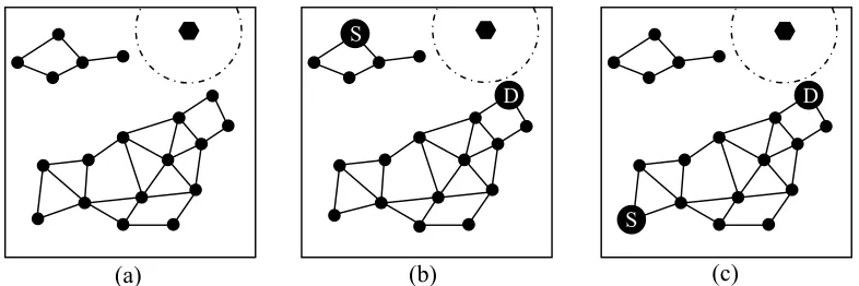
Figure 1. Different viewpoints on connectivity. (a): connectivity of whole network, (b) and (c): connectivity of two arbitrary nodes.
Recently, routing protocols in CRAHNs have gained much attraction from researchers. There have been several proposed routing protocols in CRAHNs [7-10]. Due to the limited transmission range of wireless nodes, routing paths in CRAHNs are often multi-hop paths. The challenges of routing and open research issues in multi-hop cognitive radio networks are discussed in detail in [11-12].
2. Related works and motivations
Connectivity is an important property of multi-hop paths of ad-hoc wireless networks. It is one of main factors that influence the network performance. Connectivity in traditional wireless ad-hoc network has been intensively studied in the literature. The authors in [13] investigate the probability that entire network is connected with assumption that wireless nodes have fixed circular transmission range and are distributed in disk area. In [14], the connectivity of cluster network topologies is studied. The connectivity of wireless ad-hoc network with random beamforming is presented in [15] and an analytical model for connectivity in vehicular ad-hoc networks is proposed in [16].
Nowadays, connectivity of CRAHN has raised increasing awareness of researchers. Investigating on the connectivity of multi-hop path in CRAHNs is a challenging issue compared with that of AHNs due to the random nature of node locations and PU activeness. In [17], the second smallest eigenvalue l2 of Laplacian matrix is used to evaluate the connectivity of cognitive ad-hoc networks. In [18], the second smallest Laplacian eigenvalue is also used to study the impact of only primary user on the connectivity of secondary cognitive network. The method used in [17, 18] is considered as algebraic approach. However, the drawback of the approach is that it cannot show the impact of common network parameters, such as the number of SUs and SUs, network size, network operating frequency, and the average active rates of PU, on the connectivity of CRAHNs. In addition, that method is based on static network topology with full topological information of SUs and PUs, which may not always available in
CRAHNs. Local connectivity of large scale CRAHNs, taken into account the influences of aggregated interference and beamforming were studied in [19] and [20], respectively. More importantly, the connectivity of CRAHNs in all aforementioned works is investigated in the viewpoint of connectivity of whole network (or the probability of having connected graph), and without taking into account the neighbouring node selection criteria in routing algorithm.
However, as illustrated in Figure 1, different viewpoints on connectivity may results in major difference in connectivity result. Specifically, the connectivity of whole network is 0 because the network is divided into two parts. In contrast, when we consider the connectivity between two arbitrary nodes selected as source node and destination node, the connectivity is 0 if two nodes belong to two disconnected part as in Figure 1(b) and the connectivity is 1 if two node belong to one connected part as in Figure 1(c). In addition, with routing algorithm taken into consideration, the connectivity may be different because neighboring node selection criteria makes the set of neighboring nodes different. In this paper, we study on the network connectivity of CRAHN from this perspective.
Another motivation for the work in our paper is emerged from the typical flow for evaluating the performance of routing protocols in wireless networks as in Figure 2. As shown in Figure 2, after designing routing protocols, network designers select input network parameters to evaluate the performance of these routing protocols. We observe an important fact that the performance of routing protocols in terms of packet delivery ration, throughput, delay, etc in CRAHNs and AHNs is influenced by the combined effect from many factors such as network topology related parameters (network size, the number of nodes, operating frequency, the average active rate of PU etc.), operation related parameters (routing algorithm, network congestion, random channel contention, stochastic interference, etc). Therefore, typical flow for evaluating the performance of routing protocols as in Figure 2 in a complex network environment such as CRAHNs is extremely challenging because it is difficult to determine the right factor that degrades the performance of CRAHNs. The aim of our
(a)
(b)
(c)
S
D S
D
3
Figure 2. Performance evaluation flow of routing protocols in wireless networks.
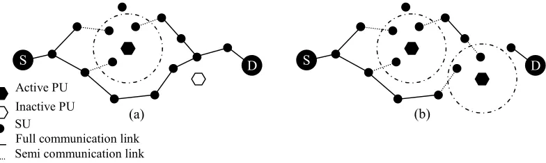
Figure 3. Network model and communication links in CRAHNs.
work in this paper is to help network designers select optimal network topology related parameters so that data transmission failures relating to network topology can be eliminated, saving network evaluation effort for network designers.
The rest of this paper is organized as follows. In Section 3, based on geographical location aware greedy routing [21], we propose algorithms to evaluate the connectivity of multi-hop path between arbitrary source node and destination node from network topology perspective with random node distribution. Section 4 shows numerical results of the connectivity of multi-hop path in CRAHNs with various simulation scenarios. Finally, conclusions and future works are given in Section 5.
3. Evaluation of the connectivity of
multi-hop path between two arbitrary nodes in
CRAHNs and AHNs
3.1. Network model
We consider CRAHNs where Ns secondary users (SUs)
coexist with Np primary users (PUs). All SUs and PUs are
uniformly distributed in network area a2. Each SU can utilize the licensed frequencies of PUs. We suppose that all PUs are characterized by an on-off transmission following Poisson distribution with average active rate
lPU. All senders transmit packets with constant power Pt
and receivers can receive packets successfully if packet reception power is higher than a threshold Pth. The
effective transmission range of wireless node is
determined by Pt, Pth, and its operating frequency. The
transmission area and forwarding area of each node are considered as circular area and semicircular area, respectively. The same network model is used for AHNs except that there are no PUs in the networks.
An illustrative example of network model and available communication links in CRAHNs is presented in Figure 3. Semi communication link is the wireless link between two nodes which are in the transmission range of each other. However, the sender is out of transmission range of active PU and the receiver is in the transmission range of active PU. Obviously, the multi-hop path from source node to destination must consist of all full communication links because all intermediate SUs on the multi-hop path in CRAHNs act as receiver and sender in order to forward data packets. In Figure 3(a), when only one PU is active, a multi-hop path can be established between source SU and destination SU. In contrast, when two PUs are active as in Figure 3(b), no multi-hop paths between these two nodes exist. Details of the method for evaluating the connectivity of multi-hop path in CRAHNs are presented below.
3.2. Our proposed algorithm
In this section, we present our proposed algorithm to evaluate the connectivity of multi-hop path from an arbitrary source node to an arbitrary destination node in AHNs and CRAHNs. With initial input network parameters such as random node location, operating frequency of wireless nodes, active state of each PU, criteria of forwarder selection (i.e. geographical location aware greedy routing [21] used in this paper), our
Performance
Evaluation
(packet delivery ratio, throughput, delay, energyconsumption, etc.)
Routing Protocols
(delay, hop count, energy, etc.)
Network
Parameters
(network size, number of nodes, operating frequency,etc.)
Active PU
Inactive PU SU
Full communication link Semi communication link
(a) (b)
D
S S D
4 proposed algorithm can check all possible paths between two arbitrary nodes considered as source node and destination node and return whether these two nodes are connected, i.e. there is at least one communication path between them. It should be noted that with the same initial input network parameters, if we apply Dijkstra’s algorithm [22] to such wireless networks, the algorithm may not work because it requires connected graph as an input. However, in AHNs and CRAHNs, due to limited transmission range, random location of wireless node (SU), and random active state of PU, there may exist no path between two arbitrary nodes. Thus, the information of connected network graph in wireless networks such as AHNs and CRAHNs is not available initially. Another issue is Dijkstra’s algorithm does not have the mechanism for determining forwarders based on routing algorithm as in our proposed path finding algorithm.
The pseudocode of our proposed algorithm used in conventional AHNs is presented in Figure 4.
The explanations for the algorithm to evaluate connectivity in AHNs with given wireless node locations are as follows:
Lines 1-2: If the destination node is within the transmission range of source node, source node can communicate directly to destination nodes without needing the support of any intermediate nodes, or the connectivity is 1. The process of finding paths is ended.
Lines 4-6: If source node does not have any neighboring nodes as forwarders, no paths from source node to destination node can be established, or the connectivity is 0. The process of finding path is also ended.
Figure 4. The pseudocode of our proposed algorithm to analyze the connectivity of multi-hop path between two arbitrary nodes in AHNs with given random wireless node locations.
1 If (d(src, dest) £ R)
2 connectivity = 1; // dest in the radio range of src® connectivity = 1
3 Else
4 fwdnode = fwdnode_chk(src) 5 If (fwdnode = {})
6 connectitvity = 0; // src does not have any forwarders ® multi-hop path cannot be established 7 Else
8 gonna_chk_node = gonna_chk_node + {fwdnode}; // add fwdnode to check list 9 hop_count(gonna_chk_node) = 1; // initialize hop count
10 While (gonna_chk_node ¹ {})
11 chk_node = gonna_chk_node; 12 For each chk_node
13 hc_chk_node = hop_count(chk_node); // get hop count to current node 14 fwdnode = fwdnode_chk(hc_chk_node); // find forwarders of current node 15 For each node Î fwdnode
16 If (node Ï already_chk_node)
17 already_chk_node = already_chk_node + {node}; // add fwd to already checked list 18 hop_count = hop_count + {hop_count(node)}; // update hop count table
19 gonna_chk_node = gonna_chk_node + {node}; // add forwarder to gonna check list
20 Else
21 If (hc_chk_node + 1 <hop_count(node))
22 hop_count(node) = hop_count(node) + 1; // increase hop count to forwarder 23 gonna_chk_node = gonna_chk_node + {node}; // add fwd to gonna check list
24 End-For
25 gonna_chk_node = gonna_chk_node \ {chk_node}; // remove checked node from the check list 26 If (dest Î already_chk_node)
27 connectivity = 1; // if dest is reached, multi-hop path can be established
28 End-For
29 End-While
30 If (dest Ï already_chk_node)
31 connectivity = 0; // multi-hop path cannot be established
5
Figure 5. The pseudocode of our proposed algorithm to analyze the connectivity of multi-hop path between two arbitrary nodes in CRAHNs with given random wireless node locations.
1 For each active PU Î PU
2 If (d(src, active PU) £ R || d(dest, active PU) £ R)
3 connectivity = 0; stop = 1; break; // src or dest is affected by active PU ® no routing path
4 End-For
5 If (d(src, dest) £ R && stop ¹ 1)
6 hop count = 1; // dest in the radio range of src® hop count = 1 7 If (d(src, dest) > R && stop ¹ 1)
8 fwdnode = fwdnode_chk(src) 9 If (fwdnode = {})
10 connectivity = 0; // src does not have any forwarders ® multi-hop path cannot be established 11 Else
12 For each node Î fwdnode 13 If (d(node, active PU) £ R)
14 fwdnode = fwdnode \ {node}; // not consider forwarders affected by active PU
15 End-For
16 gonna_chk_node = gonna_chk_node + {fwdnode}; // add fwdnode to gonna check list 17 hop_count(gonna_chk_node) = 1; // initialize hop count
18 While (gonna_chk_node ¹ {})
19 chk_node = gonna_chk_node; 20 For each chk_node
21 hc_chk_node = hop_count(chk_node); // get hop count to current node 22 fwdnode = fwdnode_chk(hc_chk_node); // find forwarders of current node 23 For each node Î fwdnode
24 If (d(node, active PU) £ R)
25 fwdnode = fwdnode \ {node}; // not consider forwarders affected by active PU
26 End-For
27 For each node Î fwdnode 28 If (node Ï already_chk_node)
29 already_chk_node = already_chk_node + {node}; // add fwd to already checked list 30 hop_count = hop_count + {hop_count(node)}; // update hop count table
31 gonna_chk_node = gonna_chk_node + {node}; // add forwarder to gonna check list
32 Else
33 If (hc_chk_node + 1 <hop_count(node))
34 hop_count(node) = hop_count(node) + 1; // increase hop count to forwarder 35 gonna_chk_node = gonna_chk_node + {node}; // add fwd to gonna check list
36 End-For
37 gonna_chk_node = gonna_chk_node \ {chk_node}; // remove checked node from the check list 38 If (dest Î already_chk_node)
39 hop count = 1; // if dest is reached, multi-hop path can be established
40 End-For
41 End-While
42 If (dest Ï already_chk_node)
43 connectivity = 0; // multi-hop path cannot be established
6 Lines 8-29: Since our proposed algorithm aims to find all possible paths from source node to destination node with given random node location, operating frequency of wireless nodes and return the connectivity of multi-hop path between these two nodes, the process of forward path searching from source node are follows: For each currently checked node, find its forwarders. These forwarders are added to the list of going-to-be checked nodes if (i) they have not been checked or (ii) the hop count from source to them is less than previous values. Node which already checked for its forwarders is removed from the list of going-to-be-checked nodes. This process is repeated for the next node in the list of going-to-be checked nodes until this list is empty.
Lines 30-31: If the list of going-to-be-checked nodes is empty but still the destination node cannot be reached, it means that no paths from source node to destination node can be established, or the connectivity is 0.
The pseudocode of our proposed algorithm used in CRAHNs is presented in Figure 5. Since PUs exist in CRAHNs, the algorithm used to evaluate the connectivity of multi-hop path in CRAHNs shown in Figure 5 has several different parts compared with the algorithm used to evaluate the connectivity of multi-hop path in conventional AHNs shown in Figure 4. Specifically, Lines 1-4: The algorithm returns the connectivity is 0 (multi-hop path cannot be established) when either source node or destination node is influenced by active PU(s). Lines 12-15 and Lines 23-26: The algorithm eliminates wireless nodes affected by active PU(s) from the list of potential forwarders because they are considered as not be able to participate in forming multi-hop path from source node to destination node. It is because the concepts of forwarders in conventional AHNs and CRAHNs are different. More specifically,
· In conventional AHNs: forwarders of a specific node are the nodes in its forwarding area.
· In CRAHNs: forwarders of a specific node are the node in its forwarding area and not affected by the presence of any active PUs.
4. Simulation analysis of the
connectivity of multi-hop path between
two arbitrary nodes in CRAHNs and
AHNs
4.1. Simulation environment and method
In this section, we present statistical simulation method to obtain simulation results of network connectivity in CRAHNs by using our proposed algorithms. We evaluate the connectivity in CRAHNs with different settings of network parameters such as the number of SUs and PUs, network size, network operating frequency, and the average active rates of PU. All wireless nodes have transmission power Pt = 10
-3
W and reception power threshold Pth = 1.58×10⁻¹² W. Those network parameters
are used for all evaluating scenarios if not further mentioned.
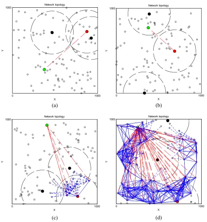
MATLAB simulation tool is used to obtain simulation results for investigating the connectivity of multi-hop path in CRAHNs. The simulation is conducted on a computer workstation equipped with 3.5 GHz (Intel Core i5 – 3570 Quad) processor, 4 GB of RAM and Windows 7. The simulation time for each value of simulation results varies from 1.4 hours to 4.9 hours, depending on the values of input network parameters such as number of wireless nodes, operating frequency of network, average active rate of PU. Figure 6 illustrates four network topologies among numerous ones randomly created during simulation with 5 PUs and 100 SUs in a network area of 1000 m × 1000 m. There is one licensed frequency layer with f = 2.4 GHz.
The detailed simulation processes are as follows.
·
Step 1: We create a square network area with size of a × a. Next, for each frequency layer, we place NSUsecondary users and NPU primary users using uniform
distribution into the network area. The number of activating times in a unit of time of each PU follows Poisson distribution with average rate lPU.
·
Step 2: One operating frequencies in the networks (i.e. licensed frequencies from PUs perspective, unlicensed frequencies from SUs perspective) are selected. The transmission ranges of wireless nodes, i.e. for both PUs and SUs, are determined by their transmission power, reception power threshold, and operating frequencies.·
Step 3: Two arbitrary SU nodes in the network are selected as source node and destination node. For each SU, a forwarding direction from it to destination node is use to determine the forwarding area, i.e. semicircular area, of that SU. If that SU has at least one neighboring SU in its forwarding region while there is no active PU in its transmission area, it is said that there is at least one communication link for that SU. The same procedure is applied for next SUs on the multi-hop path.We repeat the above processes W times for each operating frequency. For each time, a new distribution of wireless nodes is created and new arbitrary source SU and destination SU are selected. We perform the simulation of each evaluating scenario with huge number of experiments, that is, W = 50,000. Obviously, the simulation result of network connectivity of multi-hop path is calculated as
# _ SU
con
connected paths
P W®¥
¾¾¾®
W (1)
Figure 6 illustrates 4 over 50,000 random network topologies with uniform node distribution. In these random network topologies, red node is an arbitrary source SU, green node is an arbitrary destination SU, black nodes are active PUs, red dotted lines refer to the forwarding directions from current SUs to destination SU, and blue lines and blue dotted lines present full
7
Figure 6. Illustrations of 4 over 50000 random network topologies used in simulation to evaluate the connectivity of multi-hop path between two arbitrary nodes in CRAHNs.
communication links and semi communication links between two SUs, respectively. As shown in Figure 6, the multi-hop path from source SU to destination SU may not be successfully established because the following reasons: i) source SU is influenced by active PUs as in Figure 6(a), ii) destination SU is influenced by active PUs as in Figure 6(b), or iii) intermediate SUs is influenced by active PUs as in Figure 6(c). It should be noted that establishing multi-hop paths in CRAHNs may not be successful when a SU does not have any neighboring nodes in its forwarding area, as also happen in AHNs. Figure 6(d) is the case that multi-hop path is successfully established. From Figure 6(d), we can see that multi-hop path has to detour to avoid interfering with active PUs.
4.2. Numerical results and discussions
Scenario 1: The impact of node’s operating frequency on the connectivity of multi-hop path in CRAHNs and AHNs
In this scenario, we compare the point-to-point link connectivity of conventional AHNs and CRAHNs in the same network conditions. The network settings are as follows. For CRAHNs, there are 5 PUs uniformly distributed in the network area. The average activating rate of PU is lPU = 0.1. There is only one frequency layer
in the network, i.e. all PUs operate with one license frequency band and all SUs utilize that licensed frequency band to communicate with each other. The number of SUs
0 1000
1000
Network topology
X
Y
0 1000
1000
Network topology
X
Y
0 1000
1000
Network topology
X
Y
0 1000
1000
Network topology
X
Y
(a)
(b)
(c)
(d)
8 in the network is 100. All SUs are also uniformly distributed in network area. For conventional AHNs, network settings are the same as CRAHNs except that there is no PU in the network.
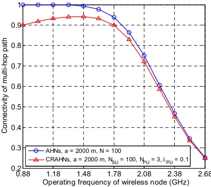
Figure 7 presents the connectivity of multi-hop path in CRAHNs as a function of wireless node’s operating frequency compared with conventional AHNs. From Figure 7, we can see some interesting features: i) the connectivity of CRAHNs is always lower than that of conventional AHN. It is due to the presence of PUs in CRAHNs, making multi-hop paths more difficult to be established. Moreover, when the operating frequency of wireless node (SU) is low (corresponding to large effective transmission range), the difference between connectivity of multi-hop path in CRAHNs and AHNs is more significant when the operating frequency of wireless nodes is high (corresponding to small effective transmission range). It is because in CRAHNs, when effective transmission range of wireless node is large, the possibility of having active PUs inside the effective transmission range of SUs is higher, leading to lower connectivity of multi-hop path. In contrast, in AHNs, there is no influence of PU’s presence on the connectivity of multi-hop path. ii) the connectivity of AHNs does not have parabolic pattern as that of CRAHNs. The reason behind this feature is there is no PU in AHNs. Whereas in CRAHN, when operating frequency of SU is low (corresponding to large effective transmission range), the possibility that an SU is influenced by active PUs strongly dominates the probability that that SU has neighboring nodes in forwarding area, resulting in low connectivity of multi-hop path. As operating frequency of SU is higher (corresponding to shorter effective transmission range), the influence of active PU’s presence is relived, leading to higher connectivity of multi-hop path. iii) when operating frequency of wireless node continues to increase (corresponding to shorter effective transmission range), the connectivity of multi-hop path in both AHNs and CRAHNs remarkably decreases and almost similar at high operating frequency of wireless node. It happens because shorter effective transmission range reduces the possibility that SU has neighboring nodes in its forwarding area and increases the hop count of multi-hop path (which also means increasing the difficulty of path establishment) at the same time.
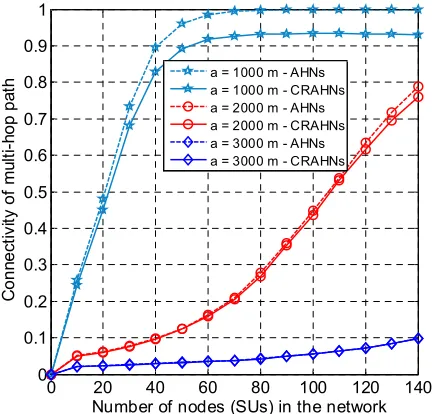
Scenario 2: The impact of the number of SUs on the connectivity of multi-hop path in CRAHNs and AHNs
In CRAHNs, a SU communicates with other SUs in the way that their communication does not interfere with the operations of PUs. Therefore, network connectivity in CRAHNs implies the connectivity among SUs in the network. In this scenario, we investigate how the number of SUs influences the network connectivity of CRAHNs provided that network size and the number of PUs are fixed. We also compare the connectivity of CRAHN with conventional AHNs when two networks have the same node (SU) density. The number of PUs in the network is 5. The average active rate lPU = 0.1. There is only one
operating frequency (i.e. one unlicensed frequency band from SU’s perspective) in the network, which is set at 2.4 GHz.
0.88 1.18 1.48 1.78 2.08 2.38 2.68
0.2 0.3 0.4 0.5 0.6 0.7 0.8 0.9 1
Operating frequency of wireless node (GHz)
C o n n e c ti v it y o f m u lt i-h o p p a th
AHNs, a = 2000 m, N = 100
CRAHNs, a = 2000 m, NSU = 100, NPU = 3, lPU = 0.1
Figure 7. The connectivity of multi-hop path in CRAHNs and conventional AHNs with different operating frequencies; network size a = 2000 m; number of SUs = 100, number of PUs = 3, average active rate of PU lPU = 0.1.
0 20 40 60 80 100 120 140
0 0.1 0.2 0.3 0.4 0.5 0.6 0.7 0.8 0.9 1
Number of nodes (SUs) in the network
C o n n e c ti v it y o f m u lt i-h o p p a th
AHNs, a = 1000 m
CRAHNs, a = 1000 m, NPU = 3, lPU = 0.1
Figure 8. The connectivity of CRAHNs compared with conventional AHNs with different numbers of wireless nodes (SUs); the number of PUs = 3, average active rate of PU lPU = 0.1, one frequency
layer with operating frequency f = 2.4 GHz.
Figure 8 shows the connectivity of CRAHNs compared with conventional AHNs as function of the number of wireless nodes (SUs). From Figure 8, the following distinguishing features can be observed: i) the connectivity of multi-hop path in both AHNs and CRAHNs rapidly increases as the number of wireless
9 nodes (SUs) increases. However, the connectivity of CRAHNs is always lower than that of AHNs due to the influence of active PUs. ii) the connectivity of multi-hop path in both AHNs and CRAHNs reach steady state when the number of wireless nodes (SUs) in higher than a certain value (i.e. 80 nodes in this simulation scenario). In steady state, the connectivity of multi-hop path is almost constant when the number of wireless nodes further increases. From this observation, we can determine the optimal number of wireless nodes which provide the highest connectivity of multi-hop path while saving network resources such as energy consumption, bandwidth usage in the networks. iii) the connectivity of multi-hop path in CRAHNs at steady state is lower than that of AHNs because active PUs occupied certain network area, thus reduces the possibility of successfully establishing routing path of SUs.
Scenario 3: The impact of node’s operating frequency on the connectivity of multi-hop path in CRAHNs and AHNs
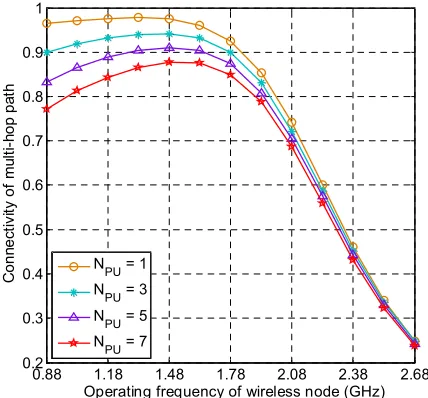
In this scenario, we study how PU’s node density affects network connectivity in CRAHNs by varying number of PUs from 1 to 7 while keeping number of SUs at 100. Average PU’s activating rate lPU = 0.1. Network size is 2000 m × 2000 m.
Figure 9 shows the connectivity of multi-hop path in CRAHNs with different number of PUs. For the purpose of evaluating the degree of influence of PU density on the connectivity of multi-hop path on different frequency bands, we plot the connectivity of multi-hop path as a function of operating frequency of wireless node and with different numbers of PUs in the networks. We can see the following important features: i) the increase in the number of PUs has stronger influence on the connectivity of multi-hop path when SU operate on low frequency bands (corresponding to large effective transmission range) compared with that when SU operate on high frequency bands (corresponding to short effective transmission range). It is because the average number of PUs in the transmission range of a SU is proportional to transmission area which depends on operating frequency of SU, ii) the parabolic relationship between connectivity of multi-hop path and the operating frequency of wireless node is significantly relaxed as the number of PUs in the networks decreases.
Scenario 4: The impact of network size on the connectivity of multi-hop path in CRAHNs
In this scenario, we study how network size affects network connectivity in CRAHNs. We use different values of network size, i.e. 1000 m × 1000 m, 2000 m × 2000 m, and 3000 m × 3000 m to create vast change of SU’s density, PU’s density, and the average distance between arbitrary source node and destination node. The number of PUs is 3. The average active rate of PU is 0.1. It should be noted that changing in network size results in changing of SU’s density, PU’s density, and the average distance between arbitrary source node and destination
node at the same time. Thus, variation in network size may have the strongest effects on the connectivity of multi-hop path in CRAHNs compared with those in previous scenarios. To provide insights of the impact of network size, we plot the connectivity of multi-hop path in CRAHNs as functions of operating frequency of wireless node and the number of SUs in the network with different network size as shown in Figure 9 and Figure 10, respectively. We also compared the connectivity of multi-hop path in CRAHNs with that in AHNs.
0.88 1.18 1.48 1.78 2.08 2.38 2.68
0.2 0.3 0.4 0.5 0.6 0.7 0.8 0.9 1
Operating frequency of wireless node (GHz)
C
o
n
n
e
c
ti
v
it
y
o
f
m
u
lt
i-h
o
p
p
a
th
NPU = 1
NPU = 3
NPU = 5
NPU = 7
Figure 9. The connectivity of multi-hop path in CRAHNs with different number of PUs; network size = 2000 m × 2000 m, number of SUs = 100, average active rate of PU lPU = 0.1, one frequency layer with
operating frequency = 0.88 GHz ~ 2.68 GHz.
As confirmed in Figure 10, changing in network size remarkably changes the pattern of the connectivity of multi-hop path. Specifically, when network size is small, i.e. a = 1000 m, the ratio of node’s effective transmission area over network size is small. Thus, the length of multi-hop path in terms of multi-hop count is short, and the possibility of finding neighboring node is high, resulting in almost perfect connectivity in AHNs. However, it may not true in CRAHNs, that is, the connectivity of multi-hop path is much lower and increases as operating frequency increase (corresponding to decrease in effective transmission range) because the influence of active PU’s is mitigated. Another interesting observation is the difference between the connectivity of multi-hop path in CRAHNs and AHs is reduced as network size increases. In addition, the connectivity of multi-hop path sharply reduces when network size a = 2000 m and a = 3000 m. It is because the ratio of node’s effective transmission area over network area decreases and the average distance between arbitrary source node and destination node rapidly increases, leading to significant increase of the path length in terms of hop count.
10
0.880 1.18 1.48 1.78 2.08 2.38 2.68
0.1 0.2 0.3 0.4 0.5 0.6 0.7 0.8 0.9 1
Operating frequency of wireless node (GHz)
C o n n e c ti v it y o f m u lt i-h o p p a th
a = 1000 m - AHNs a = 1000 m - CRAHNs a = 2000 m - AHNs a = 2000 m - CRAHNs a = 3000 m - AHNs a = 3000 m - CRAHNs
Figure 10. The connectivity of multi-hop path in CRAHNs with different network sizes; number of PUs = 3, number of SUs = 100, average active rate of PU = 0.1, one frequency layer with operating frequency = 0.88 GHz ~ 2.68 GHz.
0 20 40 60 80 100 120 140
0 0.1 0.2 0.3 0.4 0.5 0.6 0.7 0.8 0.9 1
Number of nodes (SUs) in the network
C o n n e c ti v it y o f m u lt i-h o p p a th
a = 1000 m - AHNs a = 1000 m - CRAHNs a = 2000 m - AHNs a = 2000 m - CRAHNs a = 3000 m - AHNs a = 3000 m - CRAHNs
Figure 11. The connectivity of multi-hop path in CRAHNs with different network sizes; number of PUs = 3, average active rate of PUs = 0.1, one frequency layer with operating frequency = 2.4 GHz.
The pattern of the connectivity of multi-hop path in Figure 11 also noticeably changes with different network sizes. When network size a = 1000 m, the connectivity of multi-hop path in CRAHNs and AHNs reaches saturation state as the number of nodes (SUs) exceeds certain value (80 nodes in Figure 11). In contrast, the connectivity of multi-hop paths in both CRAHNs and AHNs cannot reach saturation state when network size a = 2000 m and a = 3000m. It is due to the fact that failures in establishing multi-hop path usually occur because path length in terms
of hop count greatly increases. Especially, when network size a = 3000 m, the connectivity of multi-hop path in CRAHNs and AHNs is very low and almost similar.
Scenario 5: The impact of average active rate of PUs on the connectivity of multi-hop path in CRAHNs
In this scenario, we evaluate how the average active rate of PU influences the connectivity of multi-hop path in CRAHNs. There are 100 SUs and 3 PUs in network size of 2000 m × 2000 m. All nodes share one licensed frequency bands with frequency range from 0.88 GHz to 2.68 GHz. The average active rate of PU varies from low rate, i.e. lPU = 0.1, to high rate, i. e. lPU = 0.7.
0.88 1.18 1.48 1.78 2.08 2.38 2.68
0.2 0.3 0.4 0.5 0.6 0.7 0.8 0.9 1
Operating frequency of wireless node (GHz)
C o n n e c ti v it y o f m u lt i-h o p p a th l
PU = 0.1
lPU = 0.3
l
PU = 0.5
lPU = 0.7
Figure 12. The connectivity of multi-hop path in CRAHNs with different average active rates of PU; network size = 2000 m × 2000 m, number of SUs = 100, number of PUs = 3, one frequency layer with operating frequency = 0.88 GHz ~ 2.68 GHz.
As shown in Figure 12, the average active rate of PU has the same effect on the connectivity of multi-hop path in CRAHNs as that of the number of PUs in Figure 9. Specifically, the connectivity of multi-hop path in CRAHNs is inversely proportional to the increase of average PU’s active rate. Moreover, the parabolic pattern of connectivity of multi-hop path in CRAHNs corresponding to operating frequency of wireless node is relived as the effect of PU presence reduces, i.e. the average active rate of PU decreases.
5. Conclusions and future work
In this paper, we intensively investigate the connectivity of multi-hop path in CRAHNs by using our proposed algorithm and statistical simulation method with different network parameters such as the number of SUs and PUs, operating frequency of the network, network size, and the average active rate of PU. Unlike previous works on connectivity of in the literature, in this paper, we study the
11 connectivity of multi-hop path between two arbitrary nodes with taking the forwarder selection criteria of routing protocol into consideration, which may lead to major difference in the connectivity of multi-hop path. The simulation results obtained through various experiment scenarios with huge number of random network topologies reveal many interesting and distinguishing feature of the connectivity of multi-hop path in CRAHNs compared with that in AHNs. The results in this paper can be useful guidelines for secondary network planning, for data routing purposes and network performance to provide a reliable communication while saving network resources. Mathematical analysis of the connectivity of multi-hop paths between two arbitrary nodes in different fading channels is considered as our future work.
References
[1] F. C. Commission, (2002) Spectrum policy task force, Technical Report.
[2] MITOLA, J. I. and MAGUIRE, G. Q. (1999) Cognitive radio: making software radio more personal. IEEE Personal Communications 6(4): 13-19.
[3] AKYILDIZ, I. F., LEE, W. Y. and CHOWDHURY, F., K. R. (2009) CRAHNs: Cognitive radio ad hoc networks, Ad Hoc Networks 7(5): 810-836.
[4] MASARACCHIA, A., NGUYEN, D. L., DUONG, Q. T. and NGUYEN, M. N. (2019) An Energy-Efficient Clustering and Routing Framework for Disaster Relief, IEE Access 7: 56520-56532.
[5] KUILA, P. and JANA, K. P. (2014) CRAHNs: Energy efficient clustering and routing algorithm for wireless sensor networks: Particle swarm optimization approach, Engineering Applications of Artificial Intelligence 33: 127-140.
[6] TRAN, D. H., TRAN, T. D., LE, T. D. and CHOI, S. G. (2018) Performance Evaluation of Relay Selection Schemes in Beacon-Assisted Dual-Hop Cognitive Radio Wireless Sensor Networks under Impact of Hardware Noises, Sensors 18(6): 1-24.
[7] PARVIN, S. and FUJII, T. (2011) A Novel Spectrum Aware Routing Scheme for Multi-hop Cognitive Radio Mesh Networks. In Proceedings of 2011 IEEE 22nd International Symposium on Personal Indoor and Mobile Radio Communications (PIMRC), 572-576.
[8] CHOWDHURY, K. R. and FELICE, M. D. (2009) Search: A routing protocol for mobile cognitive radio ad-hoc networks, Computer Communications 32(18): 1983-1997. [9] CACIAPOUTI, A. S., CALEFFI, M. and PAURA, L. (2012)
Reactive routing for mobile cognitive radio ad hoc networks, Ad Hoc Networks 10(5): 803-815.
[10] LE, T. D. and AN, B. A Stability-based Spectrum-aware Routing Protocol in Mobile Cognitive Radio Ad-hoc Networks. In Proceedings of 2014 International Symposium on Computer, Consumer, and Control (IS3C), 1014-1017.
[11] CESANA, M., COUMO, F. and EKICI, E. (2011) Routing in cognitive radio networks: Challenges and solutions, Ad Hoc Networks 7(7): 228-248.
[12] SENGUPTA, S. and SUBBALAKSHMI, K. P. (2013) Open Research Issues in Multi-Hop Cognitive Radio Networks, IEEE Communications Magazine 51(4): 168-176.
[13] BETTSTETTER, C. (2004) On the Connectivity of Ad Hoc Networks, Wireless Networks 47(4): 432-447.
[14] PETROVA, M., MAHONEN, P. and RIIHIJARVI, J. (2007) Connectivity Analysis of Clustered Ad Hoc and Mesh Networks. In Proceedings of 2007 IEEE Global Telecommunications Conference (GLOBECOM '07), 1139-1143.
[15] ZHOU, X., DURRANI, S. and JONES, H. M. (2009) Connectivity of Wireless Ad Hoc Networks with Random Beamforming, IEEE Transactions on Vehicular Technology 58(9): 5247-5257.
[16] YOUSEFI, S., ALTMAN, E., EL-AZOUZI, R. and FATHY, M. (2008) Analytical Model for Connectivity in Vehicular Ad Hoc Networks, IEEE Transactions on Vehicular Technology 57(6): 3341-3356.
[17] ABBAGNALE, A., COUMO, F. and CIPOLLONE, E. (2010) Measuring the Connectivity of a Cognitive Radio Ad-Hoc Network, IEEE Communications Letters 14(5): 417-419. [18] COUMO,F., ABBAGNALE, A., GREGORINI, A. (2010) Impact
of Primary Users on the Connectivity of a Cognitive Radio Network. In Proceedings of the 9th IFIP Annual Mediterranean Ad Hoc Networking Workshop (Med-Hoc-Net), 1-8.
[19] ZHAI, D., SHENG, M., WANG, X. and ZHANG, Y. (2014) Local Connectivity of Cognitive Radio Ad Hoc Networks. In Proceedings of IEEE GLOBECOM, 1078-1090. [20] DUNG, L. T. and AN, B. (2017) A Modeling Framework
for Supporting and Evaluating Connectivity in Cognitive Radio Ad-hoc Networks with Beamforming, Wireless Networks 23(6): 1743-1755.
[21] KARP, B. and KUNG, H. T. (2000) GPSR: greedy perimeter stateless routing for wireless networks. In Proceedings of ACM MobiCom, 243-254.
[22] JOHNSONBAUGH, R. (2009) Discrete Mathematics, 7th ed. (Pearson Education, Inc.).