Soft Switching Model Predictive Control with An Increase in the Security of Calculations and Information

Soft Switching Model Predictive Control with An Increase

in the Security of Calculations and Information

Hamidreza Iranmanesh, Ahmad Afshar

*

Department of Electrical Engineering organization, Amirkabir university of Technology, Tehran, Iran. * Corresponding author. Tel.: 989335622545 email: [email protected]

Manuscript submitted May 10, 2018; accepted July 8, 2018. doi: 10.17706/jcp.13.9.1115-1126

Abstract: A popular control strategy is model predictive control. Sometimes, it is necessary to switch between multiple model predictive controllers in a plant to meet different sets of control objectives. Hard switching may introduce some unwanted effects, while the soft switching method changes to a new controller by distributing the switching process over a number of control steps, avoiding some of the hard switching problems. In this paper, a novel formulation of the soft switching coefficient in a softly switched model predictive control method is presented. This method is applied to a multi-area power system. Soft switching is performed from the initial feasible cooperation based model predictive controller to the new controller with an intentional reduction of the interaction effects on the cost function. The results of the simulation show a smaller dependence on the communication network after soft switching; therefore, the security of calculations and information is increased. Similarly, this approach can be implemented in other systems such as computer networks.

Key words: Computer network, information security, model predictive control, soft switching.

1.

Introduction

A popular control method is model predictive control (MPC) with a receding finite horizon. The basic concept of MPC is to use a dynamic model to forecast system behavior and optimize the forecast to produce the best decision for the control move at the current time [1].

Therefore, predicting the future behavior of the control variables is the principle feature of an MPC scheme [2]. The attractiveness of MPC is mostly due to its ability to directly deal with constraints, leading to safe operation of the multivariable system under all circumstances. In addition, performance criteria can be embedded into an MPC problem to improve the economics or quality of the operation [3]. The model predictive control scheme is a very helpful approach to handle time varying systems and tracking problems [4]. The core of the MPC is to replace a “closed loop optimal control” with an “open loop optimal control” in a time-varying area. As a practical alternative method, MPC has received a great deal of attention [5]. Hence, MPC has been widely used in universities and industries.

it does not usually provide satisfactory switching transients because the sudden switching may cause some unexpected impulsive phenomena such as an abrupt change of output/state, a large demand for instant control input and even actuator failure if the specifications of the two MPC controllers differ significantly [8].

The soft switching method discussed in this paper reaches the new MPC controller by distributing the switching process over a number of control steps so that the previously mentioned problems of hard switching can be avoided.

The key contributions of this paper include a novel formulation to obtain a suitable soft switching coefficient based on a presented theorem, applying the formulation to a power network, the improvement of information security by the intentional reduction of the interaction effects on the cost function and the decreasing dependence on the communication network after soft switching in a simulated power network (or similarly in a computer network).

The outline of the remainder of the paper is as follows:

The specifications of the system are explained in Section 2. Section 3 presents the optimization problem for soft switching MPC. Section 4 proposes the formulation of the soft switching coefficient and related theorem. Section 5 shows a simulation of the discussed method applied to a power network with a number of control areas. The simulation results are discussed and analyzed in Section 6. Finally, the conclusions are given in Section 7.

2.

Procedure for Paper Submission

Consider a discrete linear time-invariant system as follows:

( 1) ( ) ( )

(k) ( )

x k Ax k Bu k

y Cx k

  

 (1)

where x k( )Rn , ( )u k Rm , ( )y k Rq are state, control input and output vectors, respectively, at time k and ARn n ,BRn m , CRq n are matrix coefficients of the equations. The MPC-based controller solves the following optimization problem at each sampling time:

* _min 1_{[x ( | )Qx( | )}

0 [ (k),..., ( 1)]

T T

u ( | )Ru ( | )] x ( | )Px( | )

. .

x( 1 | ) Ax( | ) Bu( | ) , 0 1

u( | ) U , 0,1,..., 1

( 1 | ) , 0,1,..., 1

( | )

N T

J _i k i k k i k

u u k N

T

k i k k i k k N k k N k s t

k i k k i k k i k i N m

k i k R i N n

x k i k X R i N x k N k _{X f}



  _   

 

    

        

    

     

  X

(2)

where Q is a positive semi-definite matrix and R is a positive definite matrix. is an appropriately chosen terminal set and P is a semi-definite matrix that is used for weighting the terminal state. It is usually calculated offline to ensure closed-loop stability. Matrices P and K are obtained by solving the following unconstrained infinite horizon LQR problem [9], [10]:

T T

P (A + BK) P(A + BK) + K RK + Q

T -1 T

K = -(R + B PB) B PA



(3)

is the prediction horizon where Z_ is the non-negative integer numbers set. Additionally, x(k) is

feasible input sequences set are shown by U (a compact set), while the feasible states set X is a closed set.

3. Problem Statement

The important parameters in constrained MPC are matrices Q, R and P, horizon N and sets X and U.

Therefore, the problem is the soft switching from the initial MPC controller (Q_I,R_I,P N_I, _I,X_I,U_I) to the

final controller (Q_F,R_F,P_F,N_F,X_F,U_F). In the soft switching method, a sequence of intermediate MPC controllers is applied to the system and each acts as an interface between the initial and final controllers. The optimization problem of the intermediate MPC controller is as follows:

* _min 1_{[x ( | )Q x( | )}

0 [ (k),..., ( 1)]

T T

u ( | )R u ( | )] x ( | )P x( | )

s N T s

J _i k i k k i k

u u k N

s T s

k i k k i k k N k k N k



 _   

 

    

(4)

. .

x( 1 | ) Ax( | ) Bu( | ) , 0 1

u( | ) U , 0,1,..., 1

( 1 | ) , 0,1,..., 1

( | )

s t

k i k k i k k i k i N s

k i k i N

s

x k i k X i N x k N k X_f X

        

   

    

  

where (1 ) , (1 )

(1 )

s s

Q Q_I Q_F R R_I R_F

s

P P_I P_F

       

    and   k( )i is the soft switching coefficient.

Additionally, at each time step, the current state x(k)is determined and x(k|k)=x(k).

The most direct way to design constraints for the intermediate MPC is to combine the initial and final constraints in a convex manner [6]. If the soft switching coefficient   _k( )i is used to combine

constraints and the switching controller is feasible, then the following relations will be established:

(1 ) , (1 )

s s

U  U_I  U_F X  X_I  X_F (5) where X_I X U, _I U.

For each intermediate MPC controller to be feasible, its initial state must enter the intersection of the feasible sets of the previous controller and itself [6]. Thus, a constraint can be added to each intermediate MPC optimization problem to produce a feasible initial state for the next controller. For example, if the initial state of intermediate MPC controller j is at time kj, then the following constraint will be added to its

related optimization problem:

( 1| ) _{intermediate( 1)}

x k_j k_j X _j (6)

where X_{intermediate j( 1)} indicates the feasible set of intermediate MPC controller j+1.

4.

The Formulation of the Soft Switching Coefficient

The soft switching coefficient   _k( )i can be obtained based on the following theorem:

Theorem:

matrices in the performance index and N is the prediction horizon. For simplicity, the initial and final MPC controllers are assumed to have the same prediction horizon duration, that is N_I N_F N . During soft switching, the performance index is defined as follows:

1

[ ( | ) ( | )

0

( | ) ( | )] ( | ) ( | )

N

T s

x k i k Q x k i k i

T s T s

u k i k R u k i k x k N k P x

J

k N k

s  _{  }



    



_

(7)

where:

The soft switching coefficient _k( )i is obtained from the following equation:

β ( ) 1 ( ) (1 )

τ τ

k i k_b k i k_b

i H

k

sw sw

     

 _{ } 

  (8) where H is the Heaviside step function and is defined as follows:





0 0

1 1

( ) 1 ( ) 0

2 2

1 0

q

H q sign q q

q

   

  _ 

 

 

(9)

Suppose the switching begins at

k



k

_b and

τ

_sw is the switching interval.

Proof:

To transition from the initial to the final cost function, the proper coefficients should be determined for the weighting matrices:

μ₁ μ₂ , μ₁ μ₂ , μ₁ μ₂

s s s

Q  Q_I  Q_F R  R_I R_F P  P_I  P_F (10)

where

μ

₁ and

μ

₂ are suitable switching coefficients. First, the following must be true: ₁1 , ₂0 .

Accordingly, the initial weighting matrices of the cost function are achieved as follows:

s s s

Q Q , R_I R , P_I P_I for ₁1 , ₂0 (11)

At the end of the switching interval, the following must be true: As a result, the final weighting matrices of the cost function are obtained as follows:

s s s

Q Q_F , R R_F , P P_F for ₁0 ,₂1 (12)

The relationship between weighting coefficients

μ

₁and

μ

₂can be written as follows:

1 , 0 1

2 1 1

μ  μ μ  (13) Therefore, after determining how to transition one, for instance

μ

₁from 1 to 0, the formulation of the soft switching coefficient is determined. This coefficient must be decreased gradually as discrete time k increases relative to the switching start

time. The switching ends when

k



k

_e, resulting in the following:

k_ek_bτ_sw (14)

The switching coefficient is inversely related to the time interval (kk_b) such that when (kk_b) is

increased, the switching coefficient is decreased.

such that when the switching interval is shorter, the switching coefficient must be decreased faster.

If the switching process is also applied along the prediction horizon for a more realistic prediction, then the increase of variable i in x(k+i|k) over the horizon relative to the start time of the prediction is inversely related to the switching coefficient, where:

0 i N (15)

In summary, the intervalβI 1 (k i kb) τsw

 

  is inversely related to the switching coefficient; therefore,

for simplicity, we consider the following relations:

1

μ β μ₂ 1 β , ββ i_k( ) (16)

Given that 0  1, the initial formula of the switching coefficient can be presented as follows:

1 (k i kb) βI

τsw

 

  (17)

As long as0  k i k_bτ_sw, then relation 0 β 1 is established because the values of k during

switching are in the following range:

k_b k k_bτ_sw (18)

Therefore, the following inequalities will be established:

i  k i k_bτ_swi (19)

(15) and (19) result in the following:

( ) , ( ) 0

Max k i k_b τ_swN Min k i k_b  (20)

Therefore, the result is:

1

N _βI τ

_sw

   (21)

However, the switching coefficient must change from one to zero during switching. While the prediction process exceeds the switching interval, according to (21) the value of becomes negative. However, in this case, the value of the switching coefficient must be zero for the remainder of horizon, and in fact, the final controller fully applies to the system because the switching process has been completed. To solve this issue, is multiplied by the following expression in the form of a factor:

1

1 (1 )

2

k i _kb sign

τsw

 _{ }   

 

  (22)

The sign function is defined as follows:

1 0

( ) 0 0

1 0

x x

sign x x

x _x

 



  

 



So, when the initial coefficient _βI becomes negative, the value of expression (22) becomes zero. Multiplying the expression by _βI , the final value of the coefficient becomes the desired value of zero. However, if the value of _βIbecomes positive,(k i k )  _b is less than the switching interval, the switching

process has not yet finished and the value of the sign function will be one. Because of the consideration of the factor 0.5, the value of expression (22) will become one so that multiplying it by _βI has no effect.

If (k i k )  _b is equal to the switching interval, then the elapsed time relative to the switching start time

in addition to the prediction time reaches the end of the switching interval. Then, the sign function will become zero and_βI(which in this case is zero) is multiplied by expression (22) with the value of 0.5, resulting in a final value of zero.

Thus, the final formula of the soft switching coefficient is obtained as follows:

1

1 ( ) 1 (1 )

2

k i k_b k i k_b

β sign

τ_sw τ_sw

       

 _  _{ }   _

    (24)

In mathematics, the function in the second bracket is known as the Heaviside step function:

1

(1 ) 1 (1 )

2

k i k_b k i k_b

H sign

τ_sw τ_sw

 

   

  _   _

  (25)

This function is defined as follows:





0 0

1 1

( ) 1 ( ) 0

2 2

1 0

x

H x sign x x

x

  

  _ 

 _



(26)

Therefore, the soft switching coefficient can be written as follows:

( ) 1 (k i kb) (1 k i kb)

β i_k H

τ_sw τ_sw

     

 _{ } 

  (27) or

1 ( )

( )

0 k i _kb

k i k_b τ_sw τsw

β i_k

k i k_b τ_sw

 

    

    

 _{  }



(28)

Remark: If the switching coefficient is written as , then parameter  can be used as a tuning knob [8] and can change the transient performance of the switching.  0 results in hard switching and if  1, no switching will be performed. A higher value of this parameter leads to a stronger effect of the initial cost function on the switching process, while a lower value of  results in a stronger impact of the final cost function on the switching process.

5.

Simulation Study: Application to a Power Network

5.1.

Description of the Case Study

The used standard model for area j, state variables and related specifications and formulations are as follows [10]-[13] (Since automatic gain control action is limited to relatively small disturbances, the dynamics of each area can be linearized [14], [15]):

( ) / t

d PME

P_VAj P_{MEj C} dt

j

j



    (29)

( ) /

1 NE

d _{j jk}

P_ME D_{j j} P P_LD M_j

TIE

dt _k

j

j

j



 

       





(30)

( ) / t

d PVA _j

P_R P_{VA G} F

dt _rj

j

j

j

j



 _

     (31)

jk kj

P_TIE P_TIE

   (32)

TIE _{( )}

jk d P

S jk j k

dt  



    (33)

Table 1. The List of Parameters Used in the Simulation

State variables:

1 ME1 VA1

Area(1) :  , P , P Area(2) : ₂ , P_ME2 , P_VA2 , ₁₂

3 ME3 VA3 23

Area(3) :  , P , P ,  Area(4) : ₄ , P_ME4 , P_VA4 , ₃₄

Outputs: y_j ω_j j {1,2,3,4}

where the symbol Δ represents a deviation from the steady state. The list of the used parameters is given in Table 1 [11].

The initial conditions of the system are nonzero and the MPC controller drives the frequency variations to zero by solving the optimization problem and adjusting PR as the control input.

Let NP=N=50, sampling period (T)=1s, simulation time=250 and the range of control input changes is determined as follows:

0.4 0.4 , {1, 2,3, 4}

j R

P j

      (34)

Name Description Name Description

R

P load reference set point



angular frequency of system

M angular momentum  phase angle

t_G governor time constant _PME mechanical power

D (% change in load) /

(% change in frequency)

F

r (% change in frequency)/

(% change in unit output)

VA

P steam valve position

LD

P nonfrequency sensitive load

jk

S tie-line stiffness coefficient

(between areas j & k)

jk

PTIE tie-line power flow

(between areas j & k)

C

The switching times are adjusted as follows:

70 , 40 , 110

b sw e

k    k  (35)

5.2.

Architecture of System

We assume the control framework of the system is feasible cooperation-based MPC (FCMPC) that is introduced in [16]. In cooperation-based control, each controller acts to improve a global objective [17].

The FC-MPC problem of controller r can be defined as follows [10], [16]:

 





1

[ ( | ) ( | )

,

0

( | ) ( | )] ( | ) ( | )

. .

( 1 | ) ( | )

[ ₁ ( | )... ( | )... ( | )]

, 1, 2,..., ,

,

( | )

N T

u_{r N} x k i k Qx k i k i

T T

u_r k i k R u_{r r} k i k x k N k Px k N k s t

x k i k Ax k i k

T T T T

B u k i k u_r k i k u_L k i k

u_{r N} U_r r L

x k N k X J_r x k

f                       

_

(36)

where u_{r N,} [uT_r ( | )k k uT_r



k1 |k



...uT_r (k N 1 | )]k T , r1, 2,...,L

where L is the number of subsystems and the set of feasible inputs U_r is a compact set. Additionally, X_f is an invariant set including the terminal state and zero. We represent the model for subsystem r as follows:

( 1) ( ) ( ) ( ) ( )

( ) ( )

r rr r rr r rs s rs s s r

r rr r

x k A x k B u k A x k B u k

y k C x k

          _ 



₍₃₇₎

where:

( ) , ( ) , ,

, , ( ) ,

r r r r r r

r s r s r r r

n m n n n m

r r rr rr

n n n m q q n

rs rs r rr

x k R u k R A R B R A R B R y k R C R

 

  

   

   

1 2 1 2

1 2

( ) [ ( ) ( )... ( )] , ( ) [ ( ) ( )... ( )]

( ) [ ( ) ( )... ( )]

L L

L

T T T T T T T T

T T T T

x k x k x k x k u k u k u k u k y k y k y k y k

 



r

n is the number of states of subsystem r and mris the number of control inputs of subsystem r.

5.3. Description of the Problem

The goal is to switch from an initial MPC controller with complete communications between the subsystems to a new controller with an intentional reduction of the interaction effects on the cost function, causing less dependence on the communication network and, as a result, improving the security of calculations and information.

The initial and final weighting matrices for the optimization problem of controller r are generally defined as follows:

Q₁₁ Q₁₂ . . . Q_1L 0 0 . . . 0 Q₂₁ Q₂₂ . . . Q_2L 0 . . . . 0

. . . .

Q_I , Q_F

. . . . Q_rr .

. . . .

Q_L1 Q_L2 . . . Q_LL 0 0 . . . 0

                                   

P₁₁ P₁₂ . . . P_1L 0 0 . . . 0 P₂₁ P₂₂ . . . P_2L 0 0 . . . 0

. . . .

P_I , P_F

. . . . P_rr .

. . . .

P_L1 P_L2 . . . P_LL 0 0 . . . 0

                _{ } _{ }                 (38)

5.4. The Results of the Simulation

Fig. 1. The coefficient of soft switching.

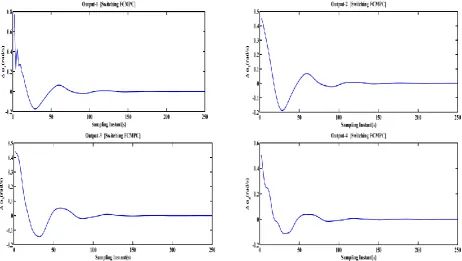
The simulation results of the switching FCMPC, including the frequency changes in the four control areas, are shown in Fig. 2.

Fig. 2. The simulation results of the switching FCMPC: a) frequency changes in area 1, b) frequency changes in area 2, c) frequency changes in area 3, d) frequency changes in area 4.

The changes of the Lyapunov function over the simulation period are depicted in Fig. 3. The Lyapunov function is as follows:

1

1 1

( ( )) [ ( ( ) ( ) ( ) ( ))] ( ) ( )

2

L k N

T T T T

i i i i i i i i i i t k

V x k x t Q x t u t R u t x k N P x k N

 

 



 

    (39)

Fig. 3. Lyapunov function.

6.

Discussion and Analysis

As shown in Fig. 2, with the nonzero initial conditions, the control method adjusts the control input to drive the frequency deviations to zero and the system reaches the steady-state after the soft switching. According to Fig. 1, the soft switching coefficient varies between one and zero. Fig. 3 shows that the Lyapunov function is decreasing over the simulation period, showing the stability of the system.

After the soft switching, the system’s dependence on the communication network is decreased and information security is increased. For illustration, to create a connection error we change the value of x2 that enters area-1 at discrete times 30 and 150 (before and after the soft switching). If x2 (the state of area-2) changes at discrete timek_c , it affectsx₁ at discrete time (k_c1)according to (37) and affects

control input-1 at (k_c1)in the optimization problem, therefore affecting output-1 at discrete time

c

(k 2).

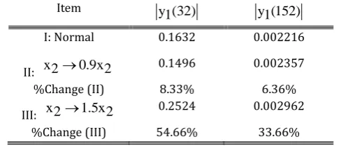
We change the value of x2 that enters area-1 in two cases: x₂0.9x₂ and x₂1.5x₂. The values of output-1 at discrete times 32 and 152 in the normal case and in two abnormal cases are reported in Table 2. The %Change is obtained as follows:

Normal value Abnormal value

%Change 100

| Normal value | 

  (40)

Table 2. The Values of Output-1 in Normal and Abnormal Cases Item

Item _{y (32)}

1 y (152)1

I: Normal 0.1632 0.002216

II: x20.9x2 0.1496 0.002357

%Change (II) 8.33% 6.36%

III: x21.5x2 0.2524 0.002962

%Change (III) 54.66% 33.66%

As shown in Table 2, %Change of y (152)1 (after the soft switching) is less than the %Change of y (32)1 (before the soft switching). Therefore, after the soft switching, the dependence on the communication network is decreased.

7. Conclusions

number of control steps, allowing some problems of hard switching to be avoided. This method was applied to a power network with four control areas. In this case study, the MPC controller drives the frequency variations to zero by solving the optimization problem and adjusting the control input. We switch softly from the initial FCMPC controller with complete communications between the subsystems to the new controller with the intentional reduction of the interaction effects on the cost function. The results of the simulation showed less dependence on the communication network after the soft switching, improving the security of calculations and information. This method can also be applied to other systems such as a computer network with multiple control areas and similar benefits can be achieved.

Acknowledgment

We would like to express our gratitude to Kerman Regional Electric Company (KREC) for preparing the relevant facilities to write this paper.

References

[1] Rawlings B., & Mayne Q. (2015). Model Predictive Control: Theory and Design, Madison, Wisconsin. Nob Hill Publishing, LLC.

[2] Akter, M., Saad Mekhilef, N., Mei T., & Hirofumi A., (2015). Model predictive control of bidirectional AC-DC converter for energy storage system. Journal of Electrical Engineering & Technology 10(1),

165-175.

[3] Vojtech V., & Danica R. (2014). Robust MPC controller design for switched systems using multi-parameter dependent lyapunov function. International Journal of Innovative Computing, Information and Control, 10(1), 43-51.

[4] Lee, S. (2009). Robust model predictive control using polytopic description of input constraints.

Journal of Electrical Engineering and Technology, 4(4), 566-569.

[5] Wang, S., Junyong F., Ying Y., & Jian S. (2017). An improved predictive functional control with minimum-order observer for speed control of permanent magnet synchronous motor. Journal of Electrical Engineering and Technology, 12(1), 272-283.

[6] Wang, J., & Brdys A. (2006). Supervised robustly feasible soft switching model predictive control with bounded disturbances. Proceedings of the 6th World Congress on Intelligent Control and Automation.

[7] Lixian Z., Songlin Z., & Richard D. (2016). Switched model predictive control of switched linear systems: Feasibility, stability and robustness. Automatica, 67, 8–21.

[8] Jingsong W. (2006). Supervised robustly feasible soft switching model predictive control with polytopic uncertainty. Proceedings of the First International Conference on Innovative Computing, Information and Control (ICICIC'06).

[9] Mayne, D. Q., Rawlings, J. B., Rao, C. V., & Scokaert, P. O. M. (2000). Constrained model predictive control: Stability and optimality. Automatica, 36, 789–814.

[10]Hermans M., Jokic A., Lazar M., Alessio A., van den Bosch P. J., Hiskens A., & Bemporad A. (2012). Assessment of non-centralized model predictive control techniques for electrical power networks.

International Journal of Control,85(8), 1162–1177.

[11]Aswin N., Ian A., Rawlings B., & Wright J. (2008). Distributed MPC strategies with application to power system automatic generation control. IEEE Transactions on Control Systems Technology,16, 6.

[12]Wood A. J., & Wollenberg B. F. (1996). Power Generation Operation and Control, New York: Wiley. [13]Kundur, P. (1994). Power System Stability and Control, New York, NY, USA: McGraw-Hill.

[15]Venkat, N., Rawlings B., & Wright, J., (2005). Stability and optimality of distributed model predictive control. Proceedings of the 44th IEEE Conference on Decision and Control and the European Control Conference, 12-15.

[16]Venkat, A. N. (2006). Distributed Model Predictive Control: Theory and Application. Ph.D thesis, University of Wisconsin-Madison.

[17]Stewart, B. (2010). Plantwide Cooperative Distributed Model Predictive Control. Doctor of philosophy dissertation, University of Wisconsin–Madison.

Hamidreza Iranmanesh received the B.S. degree in electrical engineering from the Khaje

Nasir Toosi University of Technology, Tehran, Iran, in 1993 and the M.S. in electrical engineering from University of Guilan, Iran, in 1997. He is currently pursuing the Ph.D. degree in electrical engineering at Amirkabir University of Technology (Tehran Polytechnic), Tehran, Iran. Since 1999, he has been with Ministry of Energy of Iran (KREC). He has worked in the fields of electric demand-side management, technical planning and design of electronic circuits. His research interests include model predictive control, large-scale systems, stability, demand response and energy management. He is a member of Iranian Association of Electrical and Electronics Engineers (IAEEE). He has been also a member of the editorial board of the

electronic journal of IAEEE (Kerman branch) and a member of Iranian Network of Energy Friends.

Ahmad Afshar received his Ph.D degree in electrical engineering from Manchester University in 1991 and subsequently started his career as a member of staff with University of Petroleum in the department of Electrical Engineering. He joined Amirkabir University of Technology in 1998.