©IJRASET 2015: All Rights are Reserved
358
Frequent Items Mining in Data Streams
Dr. S. Vijayarani1, Ms. R. Prasannalakshmi2
1
Assistant Professor, 2M.Phil Research Scholar, Department of Computer Science,
School of Computer Science and Engineering, Bharathiar University, Coimbatore, Tamilnadu, India.
Abstract - The main goal of this research is to mine frequent items in data streams using ECLAT and Dynamic Itemset Mining algorithms and finding the performance and drawbacks of these two algorithms. Most commonly used traditional association rule mining algorithms are APRIORI algorithms, Partitioning algorithms, Pincer-Search algorithms, FP-Growth Algorithms and Dynamic Item Set Mining Algorithms, Eclat algorithms and so on. The performance factors used are number of frequent items generated using different thresholds and execution time. From the experimental results we come know that the performance of Éclat algorithm is better than the Dynamic Item Set Counting Algorithm.
Keywords - Data streams, Association rules, Frequent Items, Éclat algorithm, Dynamic Item Set Counting Algorithms.
I. INTRODUCTION
Advanced developments in the hardware industry have provided the organizations to store and process huge flow of transactional data. These types of data sets which endlessly and quickly grow over time are known as data streams. Nowadays, real time events are monitored with the help of sensor technology which creates a platform to store this information in the databases. In order to handle these databases, i.e. to mine or knowledge extraction is not possible by using the traditional data mining algorithms. In many cases, these large volumes of data can be mined for interesting and relevant data stream information in a wide variety of applications [1]-[2].
This research work mainly concentrated on generating frequent items which is the first and essential step of association rule generation. From these frequent items only, the association rules are generated. This work helps to generate the frequent items in data streams using existing association rule data mining algorithms. Popular association rule generation algorithms, ECLAT and DIC are used and its performances are compared by using the factors number of rules generated and execution time The paper is organized as follows. Section 2 provides the related works. Proposed methodology and the traditional association rule mining algorithms are given in Section 3. Section 4 described the experimental results. Conclusion is given in Section 5.
II. REVIEWOFLITERATURE
Vijayarani S et al., [17] described frequent item-set mining in data streams. Authors have used ECLAT and RARM algorithms for generating the frequent item-sets. The dataset was divided into number of windows with different threshold values. The performance factors used are number of frequent items generated and execution time. From the results, the authors observed that the performance of ECLAT is more efficient than RARM.
Vijayarani S et al., [18] performed a comparative analysis of traditional association rule mining algorithms for data streams. The algorithms considered for analysis are APRIORI, APRIORI PT (Prefix Tree) and APRIORI MR (Map/Reduce). Different sizes of windows and threshold values are used and it is concluded that APRIORI MR has produced good results than other algorithms.
Charu C. Aggarwal, [4] presented the complete information about data streams. He discussed how to relate variant data mining technologies to data streams for supportive and unknown data extraction. He also discussed data stream clustering, data stream classification, association rule mining algorithm in data stream and frequent pattern mining.
Preeti Paranjape-Voditel et al., [11]-[8] discussed the distributed algorithm based on DIC algorithm for frequent item generation. It is based on APRIORI algorithms in the number of single pass of the databases and which is used to represent the different methods in distributed association rule mining algorithms. From the performance evaluation, the distributed DIC algorithm is efficient in dense data set and reduced the execution time.
Bin et al., [4]-[14] described the DIC algorithms in association rule mining. Author explained the real time number of passes of the databases in certain computations and which is used to represent the different methods in association rule mining algorithms. Author used different types of structures and this structure can be associated from single passes.
©IJRASET 2015: All Rights are Reserved
359
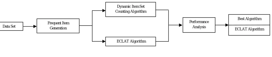
III. PROPOSEDMETHODOLOGY [image:3.612.71.544.139.238.2]The system Architecture of this work is given in Figure 1.
Fig. 1 System architecture A. Dataset
The connect data set is used in this work. It is taken from http://fimi.ua.ac.be/data/connect.dat. It consists of 67,558 instances and 48 attributes. From this 1K, 2K and 5K transactions are used in this work. In data streams, we have assumed that the nonstop arrival of data is divided into many windows with permanent size, i.e. W1, W2, W3...Wn. In this work, we have created five windows W1, W2, W3, W4, W5 with the static data set size of 1K, 2K and 5K.
B. Association Rule using Frequent Items Generation
The frequent item generation is used in association rule mining algorithms. Let, the sample data set D be a number of transactional item, i.e. D = {I1, I2, ….. I (D)}. Let X be the set of all frequent interesting patterns occurring in database D, g be a counting function like g: X * D -> N, Where I is the number of transactions, and N is the set of non-negative integers. Given parameters p ∪ X and i ∪ I, g(p,i) returns the amount of transactional time occurs in i.
The support of a pattern p Xin the data set D is defined by,
( ) = Y(g(p, I ))
The frequent item is an item generation which frequently occurred in a transaction. Frequent item set mining is used to discover the patterns in customer transaction databases. These types of transactional databases are used in business organizations and supermarkets for taking important decisions. The algorithms used here are,
1. ECLAT Algorithm. 2. DIC Algorithm.
C. ECLAT Algorithm.
Equivalence Class Clustering and Bottom up Lattice Traversal is an acronym for ECLAT algorithm. The name implies that the algorithm uses the bottom up searching method like as horizontal and vertical layouts to find out the frequent item set. This algorithm also performed the item set mining. It uses the tid set of intersection to compute the support of the candidate item set and it is compared with other algorithms like Apriori , FP-growth, Partitioning algorithm, Apriori Map/Reduce, Apriori PT, frequent items, Supervised Association rules and Association outliers algorithm, etc., It required the candidate generation phases and pruning phases.
There are two important steps in ECLAT algorithm. First one is, candidate generation and the second one is pruning. In the candidate generation step, each k-item sets candidate is produced from two frequent (k-1) – item sets and then its support is calculated, if it considered as supported value is lesser than the threshold values, then it will be discarded, otherwise it is frequent item-sets and used to (k+1) – item sets. Because, the ECLAT algorithm uses the vertical layout, counting support is unimportant. Candidate generation is really a search in the search tree. This search is a depth-first search and it begins with frequent items in the item base and then 2 – item setsare reached from 1- item sets, 3 – item sets are reached from 2 – item sets
Data Set Frequent Item Generation
ECLAT Algorithm
Performance Analysis
Best Algorithm
ECLAT Algorithm Dynamic Item Set
360
and so on.
1) Candidate Generation : A k- item set is generated by taking the union of two (k-1) – item sets which have (k-2) item sets at
[image:4.612.154.457.233.383.2]frequent, the two (k-1) –item sets are called parent item sets of the k-item set. For example, {{abc} = {ab} {ac}}, {ab} and {ac} are parent of {abc}. To avoid generating duplicate item sets, (k-1) – item sets are sorted in some order. For example, we have a set of 1 – item sets {a,b,c,d,e}, which share 0 items and sort items in the alphabet order; to generate all 2 – item sets, union of {a} with {b,c,d,e}to result 2-itemsets {ab,ac,ad,ae}, then it take union of {b} with {c,d,e} to have {bc,bd,be}, similarly, for {c} and {d}; lastly, get all possible, 2- item sets {ab,ac,ad,ae,bc,bd,be,cd,ce,de}; generate all feasible 3-itemsets from these 2-3-itemsets. Initially have divided these item sets into groups, anywhere each group has a common item; in each group, to generate feasible 3-itemsets from that group, then collecting all 3-itemsets generated from groups, all possible 3-itemsets from the item base {a,b,c,d,e}.The search tree of an item base {a, b, c, d, e} is represented by the tree as below:
Fig. 1 Searching tree for frequent item based
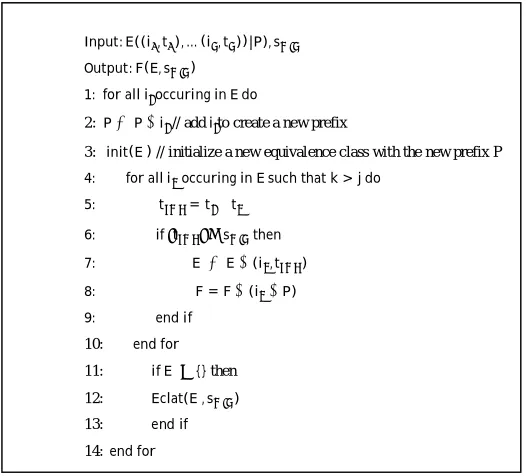
2) Pseudo Code for ECLAT Algorithm
Fig. 3 Pseudo code for ECLAT algorithm Input: E((i , t ), … (i , t ))|P), s
Output: F(E, s )
1: forallioccuringinEdo
4: foralli occuringinEsuchthatk > jdo 5: t = t∩t
6: if t ≥s then 7: E′≔E∪(i , t )
8: F = F∪(i ∪P) 9: endif
2: P≔P∪i // add ito create a new prefix 3: init(E′)
// initialize a new equivalence class with the new prefix P
10: endfor
11: ifE′≠{}then
12: Eclat(E′, s )
13: endif
[image:4.612.174.437.439.677.2]©IJRASET 2015: All Rights are Reserved
361
D. DIC Algorithm
Dynamic Item Set Counting Algorithm is proposed by Bin et al. in 1997. The validation behind DIC works like a train running over the data, with stops at intervals N between Numbers of transactions. When the train arrives at the end of the transaction file, it has made one pass over the data, and it starts all over again from the starting for the next pass. The passengers on the train are item sets. While an item set is on the train, count its occurrence in the transactions that are interpreted. When an APRIORI algorithm is considered in all item sets get on at the start of a pass and get off at the end. The 1 – item sets obtained the first pass, the 2 – item sets obtain the second pass, and so on. In DIC, there is the added flexibility of allowing item sets to get on at any stop as long as they get off at the same stop the next time the train goes around. Therefore, the item set has seen all the transactions in the file.
Consider the DIC example, imagine 40,000 transactions and N = 10,000. It will count all the 1 – item sets in the first 40,000 transactions. Though, begin counting 2 – item sets after the first 10,000 transactions have been interpreted. It will begin counting 3 item sets after 20,000 transactions. To assume that 4 – item sets need to count. It will be getting to the end of the file and top counting the 1 – items sets and go back to the start of the file to count the 2 – and 3 – item sets. After the first 10,000 transactions and finish counting the 2 – item sets and after 20,000 transactions, finally finish counting the 3 – item sets. In total, have made 1.5 passes over the data in its place of the 3 passes a level – wise algorithm would build.
1) Structure of DIC: Dynamic Item Set Counting Algorithm has defined by four different structures like as, Dashed Box,
Dashed Circle, Solid Box, and Solid Circle. Each of these structures maintains a list of item sets. It gives a two important factors are used, that is Dashed and Solid Categories.
This item sets in the “dashed” category of structures has a counter and discontinue number with them.
a) The counter is to maintain track of the support value of the corresponding item set.
b) The stop number is to maintain track whether an item set has fulfilled one full pass over a database. c) The item sets in the “solid” category structures are not subjected to any counting.
d) The item set in the solid box is an established set of frequent sets. e) The item sets in the solid circle are the established set of infrequent sets.
f) The algorithm counts the supported values of the item sets in the dashed structure as it moves along from one stop point to another.
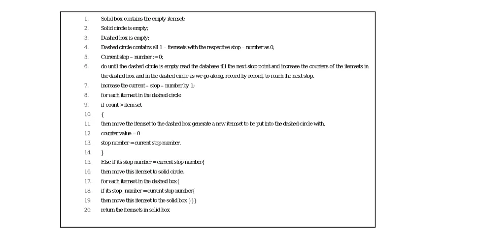
[image:5.612.63.548.461.698.2]2) Pseudo Code for DIC Algorithm:
Fig. 4 Pseudo code for DIC algorithm
1. Solid box contains the empty itemset;
2. Solid circle is empty;
3. Dashed box is empty;
4. Dashed circle contains all 1 – itemsets with the respective stop – number as 0;
5. Current stop – number := 0;
6. do until the dashed circle is empty read the database till the next stop point and increase the counters of the itemsets in
the dashed box and in the dashed circle as we go along, record by record, to reach the next stop.
7. increase the current – stop – number by 1;
8. for each itemset in the dashed circle
9. if count > item set
10. {
11. then move the itemset to the dashed boxgenerate a new itemset to be put into the dashed circlewith,
12. counter value = 0
13. stop number = current stop number.
14. }
15. Elseif its stop number = current stop number{
16. then move this itemset to solid circle.
17. for each itemset in the dashed box{
18. if its stop_number = current stop number{
19. then move this itemset to the solid box }}}
©IJRASET 2015: All Rights are Reserved
362
During the execution of the DIC algorithm, at any stop point, the following events take place,
1) Certain item sets in the dashed circle move into the dashed box. These are the item sets whose support – counts reach value during this iteration (reading records between two consecutive stops).
2) Certain item sets enter the system and get into the dashed circle. These are essentially the supersets of the item sets that move from the dashed circle to the dashed box.
3) Item sets that have completed one full pass move from the dashed structure to a solid structure. That is, if the utmost is in a dashed circle while completing a full pass, it moves into the solid circle. If it is in the dashed box, then it moves into a solid box after completing a full pass.
IV. EXPERIMENTALRESULTS
The experimental results of ECLAT and DIC algorithms are described in this section. The work is implemented in MySQL Query Browser and Java IDE Environments. Totally, five windows W1, W2, W3, W4 ,W5 are used in this research work. Thereare four different sizes of datasets; 1K, 2K, 5K, 10K is tested and their results are obtained. Different threshold values are applied for analyzing the results. The performance factors used for analysis are number of rules generated and execution time.
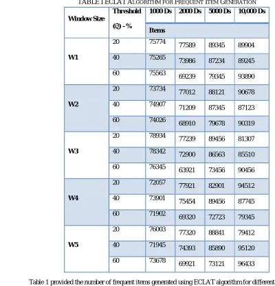
[image:6.612.63.463.289.706.2]TABLEIECLATALGORITHM FOR FREQUENT ITEM GENERATION
Table 1 provided the number of frequent items generated using ECLAT algorithm for different threshold values i.e.
= 20,40,60. This is represented in Fig. 5
Window Size
Threshold
( ) - %
1000 Ds 2000 Ds 5000 Ds 10,000 Ds
Items
W1
20 75774 77589 89345 89904
40 75265
73986 87234 89245
60 75563
69239 79345 93890
W2
20 73734
77012 88121 90678
40 74907 71209 87345 87123
60 74026 68910 79678 90319
W3
20 78934 77239 89456 81307
40 78342 72900 86563 85510
60 76345
63921 73456 90456
W4
20 72057 77921 82901 94512
40 73901 75454 89456 87745
60 71902 69320 72723 79345
W5
20 76003 77320 88841 79412
40 71945 74393 85890 95120
[image:6.612.73.455.290.702.2]363
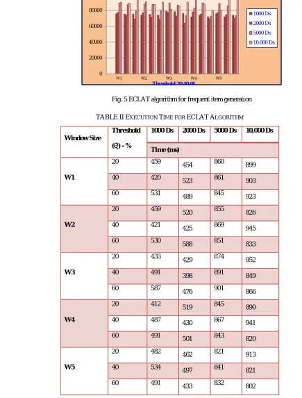
Fig. 5 ECLAT algorithm for frequent item generation
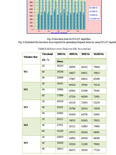
TABLEIIEXECUTION TIME FOR ECLATALGORITHM
Table 2 represented the execution time required for generating frequent items by using ECLAT algorithm.
0 20000 40000 60000 80000 100000 120000
W1 W2 W3 W4 W5
1000 Ds
2000 Ds
5000 Ds
10,000 Ds
ECLAT Algortihm for Frequent Item Generation
Threshold 20,40,60
Window Size
Threshold
( ) - %
1000 Ds 2000 Ds 5000 Ds 10,000 Ds
Time (ms)
W1
20 459
454 860 899
40 420 523 861 903
60 531
489 845 923
W2
20 459 520 855 826
40 421 425 869 945
60 530
588 851 833
W3
20 433
429 874 952
40 491
398 891 849
60 587 476 901 866
W4
20 412 519 845 890
40 487 430 867 941
60 491 501 843 820
W5
20 482 462 821 913
40 534 497 841 821
60 491
364
Fig. 6 Execution time for ECLAT algorithm
Fig. 6 illustrated the execution time required for generating frequent items by using ECLAT algorithm.
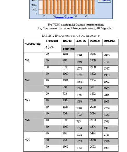
TABLEIIIEXECUTION TIME FOR DICALGORITHM
Table 3 represented the frequent item generation using DIC algorithm for different threshold values i.e. = 20,40,60.
0 100 200 300 400 500 600 700 800 900 1000
W1 W2 W3 W4 W5
1000 Ds
2000 Ds
5000 Ds
10,000 Ds
Execution Time for ECLAT Algorithm
Threshold 20,40,60
Window Size
Threshold
( ) - %
1000 Ds 2000 Ds 5000 Ds 10,000 Ds
Items
W1
20 40210
44992 64322 79944
40 59198 44827 69451 79823
60 55069
57867 60812 65290
W2
20 58161 60418 59345 76120
40 29944 62902 61998 79345
60 57898 47550 60569 72901
W3
20 44519 43120 51816 53234
40 45221
55780 62010 72938
60 61665
62439 64756 55902
W4
20 65211
54832 65443 78432
40 47551 45121 52983 73965
60 41229 47672 68344 69091
W5
20 62819
43892 60528 84589
40 59320
59320 51290 79943
60 49413
365
Fig. 7 DIC algorithm for frequent item generations Fig. 7 represented the frequent item generation using DIC algorithm.
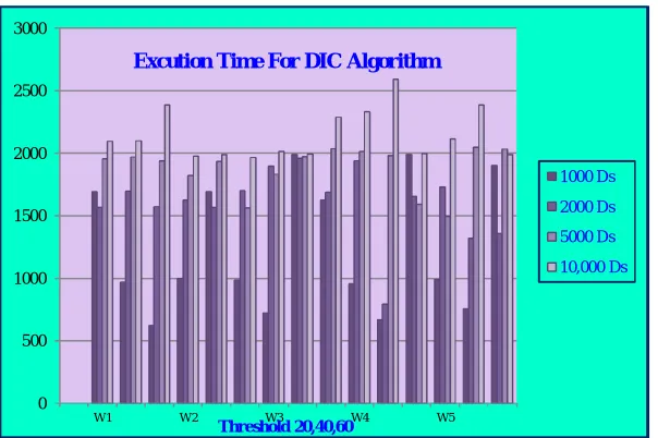
[image:9.612.62.498.176.698.2]TABLEIVEXECUTION TIME FOR DICALGORITHM
Table 4 shows the execution time required for generating items by using DIC algorithm for different threshold values
0 10000 20000 30000 40000 50000 60000 70000 80000 90000
W1 W2 W3 W4 W5
1000 Ds
2000 Ds
5000 Ds
10,000 Ds
DIC Algorithm for Frequent Item Generations
Threshold 20,40,60
Window Size
Threshold
( ) - %
1000 Ds 2000 Ds 5000 Ds 10,000 Ds
Time (ms)
W1
20 1691
1564 1956 2096
40 967
1694 1969 2101
60 619
1573 1938 2387
W2
20 1000 1623 1822 1980
40 1691 1565 1934 1992
60 988
1699 1561 1965
W3
20 723 1897 1832 2014
40 1989
1958 1976 1995
60 1625
1687 2038 2289
W4
20 954
1938 2014 2332
40 670 793 1983 2591
60 1990 1654 1594 1997
W5
20 991 1732 1494 2115
40 754 1322 2048 2389
60 1902
[image:9.612.128.468.311.698.2]366
[image:10.612.157.459.95.296.2]i.e. = 20,40,60.
Fig. 8 Execution time for DIC algorithm
Figure 8 shows the execution time required for generating items by using DIC algorithm
V. CONCLUSIONANDFUTUREWORK
From this work, it is concluded that the performance of ECLAT algorithm is better than DIC algorithm. ECLAT algorithm has generated more number of frequent items with different thresholds and different sizes of data sets. The execution time required to generate frequent items by ECLAT is also less than DIC algorithm. In future, association rules are generated by using the enhanced versions of these algorithms.
REFERENCES
[1] Aggarwal C. “A Framework for Diagnosing Changes in Evolving Data Streams”. ACM SIGMOD Conference, 2003.
[2] Agrawal, R. and Srikant, R. “Fast Algorithms for Mining Association rules”. Proceedings, 20th VLDB conference, Santiago, Chile, 1994.
[3] A. Savasere, E. Omiecinski, and S.B. Navathe, “An efficient algorithm for mining association rules in large databases,” International Conference on Very Large Databases, PP: 432–444, 1995.
[4] Bin et al., “ Dynamic Itemset Counting Algorithms”, 1997.
[5] Charu C. Aggarwal “Data Stream Models and algorithms”- Book for Data stream, Springer, 2009. [6] Arun k Pujari “Data mining techniques “, 2008.
[7] Charu C. Aggarwal “Data Streams: An Overview and Scientific Applications”. [8] Margaret H. Dunham “Data Mining: Introductory and Advanced Topics” [9] Frequent item set mining data set repository, http:// fimi.cshelsinki.fi/data/ \
[10] Han, J., Kamber, M.: “Data Mining Concepts and Techniques”, Morgan Kaufmann Publishers, 2006.
[11] Preeti Paranjape-Voditel, Dr.Umesh Deshpande, “A DIC-based Distributed Algorithm for Frequent Itemset Generation” Journal Of Software, Vol. 6, No. 2, February 2011.
[12] Rakesh Agrawal, Ramakrishnan Srikant, “Fast Algorithms for Mining Association Rules” International Conference on Very Large Databases, September 1994.
[13] S.Vijayarani, P.Sathya, “ Mining Frequent Item Sets over Data Streams using Éclat Algorithm” , International Conference on Research Trends in Computer Technologies (ICRTCT - 2013) Proceedings published in International Journal of Computer Applications® (IJCA) (0975 – 8887) 27.
[14] S.Brin and R.Motwani and J.Ullman and Shalom Tsur, “Dynamic Itemset Counting and Implication Rules for Market Basket Data” ,SIGMOD Record, volume 6,number 2,pages 255-264,June 1997.
[15] Tannu Arora1, Rahul Yadav2 “Improved Association Mining Algorithm for Large Dataset”, IJCEM International Journal of Computational Engineering & Management, Vol. 13, July 2011 ISSN (Online): 2230-7893.
0 500 1000 1500 2000 2500 3000
W1 W2 W3 W4 W5
1000 Ds
2000 Ds
5000 Ds
10,000 Ds
Excution Time For DIC Algorithm