Flow Analysis of a Symmetrical Channel with Multiple Jets at the Upper Wall

Flow Analysis of a Symmetrical Channel with Multiple

Jets at the Upper Wall

Nuri Kayansayan

Department of Mechanical Engineering, Near East University Turkey

Received October 15, 2019; Revised November 26, 2019; Accepted December 4, 2019

Copyright©2020 by authors, all rights reserved. Authors agree that this article remains permanently open access under the terms of the Creative Commons Attribution License 4.0 International License

Abstract

The objective of this study is to analyze experimentally and numerically the flow characteristics of a symmetric channel arisen from flow modeling of the blade cooling problem. The two ends of the flat channel are open and five evenly spaced air jets of equal strength at the upper wall configure a symmetrical flow around the mid-slot symmetry axis. The parameters that govern the flow characteristics of such a system are; the channel height, the jet spacing, and the jet velocity. In the analysis, the slot width is kept constant, but the channel height to slot width ratio (

H

/



), and the slot spacing ratio (

s

/



) vary in the range of 1-3 and 2-4 respectively. In addition, the flow Reynolds number (Re) is altered in a range between 1500 and 10500 for each channel geometry of nine combinations. In experiments, the pressure distributions by an electronic micro-manometer, and the velocity profiles by a hot-wire anemometry system are measured. In numerical approach, the realizable k−ε turbulence model with enhanced wall treatment is used for the turbulence computations. Comparisons with the experimental data obtained under isothermal conditions allow evaluation of the performance of the numerical model. The results show that the channel height is the dominant parameter that affects the flow characteristics and a correlation is proposed for determining the pressure drop coefficient of the injection section.

Keywords

Channel Flow, Impingement,

Computational Fluid Dynamics, Turbulence

1. Introduction

Due to removing high heat flow rates, impinging jets have been employed for many engineering applications. Ebadian and Lin (2011) compared the different methods of high-heat flux heat removal including micro-channels, jet impingements, sprays, wettability effects, and

point heat transfer rates of the downstream jet decreased by about 30-percent. Özmen (2011) performed an experimental study to investigate the effect of nozzle-to-plate spacing, jet-to-jet spacing, and the Reynolds number on pressure distribution for a confined twin impinging jet at high Reynolds numbers. It was found that pressure distribution was a function of both nozzle-to-plate spacing and jet-to-jet spacing. Afroz and Sharif (2013) numerically investigated the flow structure resulting from two-dimensional turbulent twin oblique and confined slot jet impinging at the upper wall. In their analysis, the pressure distribution of the channel and the variation of skin friction coefficients along the impingement surface were presented. Forouzanmehr et al. (2015) developed a numerical algorithm to obtain the optimal configuration of four planar impinging slot jets to produce uniform heat flux along isothermally heated flat plate. Similarly, the flow characteristics of low speed quadruple slot jet arrays is analyzed by Shariatmadar et al. (2015; 2016). In the analysis, jet-to-plate spacing varied from 26.4 mm to 27.6 mm, slot width in the range of 2-5 mm, and jet-to-jet spacing is taken to be between 2 mm to 3 mm. It is evident from literature that the flow characteristics of multiple impinging jets can differ substantially from those of a single jet. Essentially two types of interactions that do not occur in single jet systems can affect the individual jets of a multi-jet configuration. The first is the possible jet-to-jet interaction between pairs of adjacent jets prior to their impingement onto the target plate. Slayzak et al. (1994) experimentally found local maximum heat rates between jets in an array of two slot jets at height and spacing ratios ofH /=17.4, s/=10 respectively and the result was attributed to jet interaction. Secondly, there is the interaction between the impinging jets due to flow of spent air formed by the neighboring jets. These disturbances predominantly affect the heat transfer for arrays with small inter-jet spacing, small separation distances, and large jet velocities (Huber and Viskanta, 1994; San and Lai, 2001).

In the present analysis, the curvature effects of the airfoil contour as in Fig. 1a may be neglected based on the

reasoning that series of jets impacted into the blade inner surface give rise to the localized thinning of the boundary-layer type flow near the impact points. Besides, the formation of recirculation zones in the flow and merging of jets would result with high-order influence than those caused by airfoil curvature (Zuckerman et al., 2005; Han et al., 2006).

As depicted in Fig. 1b, the objective of this paper is to study the influence of slot jet geometry specifically; jet-to-jet spacing and the channel height, and the jet flow rate on the hydrodynamic behavior of a symmetric channel flow caused by confined and normally impinging, equally spaced five air jets at the upper wall. Such a configuration simulates the general features of internal cooling of a turbine airfoil exposed to high-temperature stream. In the analysis, the flow Reynolds number ( Re ) and the slot hydraulic diameter,

d

_h are defined respectively as follows,

Re

ρ

V dj h

µ

= and

d

_h

=

2



(1)

The channel general dimensions together with the slot spacing and the channel height variations that are used in both experiments and numerical analysis are presented in Fig. 1. Moreover, the jet Reynolds number ( Re ) is varied in the range between 1500 and 10500 at each specified channel geometry and the velocity flow field and pressure drop characteristics are analyzed through local hot-wire and pressure measurements. A detailed description of the experimentation and measurement techniques, along with the data reduction and definition of experimental uncertainties, is provided prior to numerical analysis. ANSYS FLUENT 17 commercial CFD code is used for numerical study of the flow domain specified by the slot pitch and the channel height ratio. The computed results for nine different geometric combinations are presented in terms of the streamlines, velocity, and pressure distributions across the channel and are meant to serve as comparison with the experimental data.

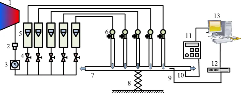
[image:2.595.127.466.570.741.2]

Figure 2. Schematic diagram of the experimental setup: 1.Air compressor, 2.Air dryer, 3.Pressure regulator, 4. Flow rate adjustment, 5.Rotameter, 6.Air plenum, 7.Test section, 8.Vertical moving unit and stage controller, 9.Hot wire probe, 10.Pressure measuring system, 11. Data acquisition unit, 12.Hot wire anemometry, 13.PC and data acquisition software

2. The Experiments

2.1. Jet Generation and the Experimental Set-up

A schematic of the experimental apparatus is presented in Fig. 2. The air jet was generated by a compressor facility and was directed to a desiccant dryer to eliminate any moisture content. The facility was capable of supplying 190Ls-1 of air to the test section at full load conditions. Following the pressure regulator, air was supplied to the system at a constant pressure of 7 bar and at a temperature of 21oC.

Before entering a rotameter, a needle valve provided the desired flow rate on that particular airline. The rotameter exit was connected to 25 mm diameter pipe for span-wise distribution of air at the plenum inlet. Each injection slot of the upper wall of the experimental channel had the dimensions of 580 mm 12.7 mm× and was sufficiently long to produce steady and uniform velocity profile at the exit surface of the air plenum (Pope, 2013).

Through a calibration process, the flow uniformity at the slot exit was assured with a maximum deviation of

2.5%

± from the average velocity at high flow rates. The distance between the adjacent slots was varied by aluminum spacers placed on pre-machined grooves on the plenum sidewalls. The smoothness of the injection surface (the channel upper wall) was secured by mounting the plenums on a relatively rigid frame and by keeping the size tolerance of interconnected parts minimum. Leakage between the spacers forming the upper wall was prevented by the application of liquid sealant to the interfaces. The channel lower wall was an aluminum plate with dimensions of 1000 mm×660 mm×6 mm. A total of 41 pressure taps 0.8 mm in diameter with a special configuration as to reduce the reading error to a minimum (Chue, 1975) were machined on the symmetry line staggered with 12 mm off from the centerline. Due to steep change of pressure around the stagnation point, 14 taps close to this region were 14 mm apart, and the others were

[image:3.595.93.509.82.246.2]

28 mm apart. The pressure tap of the stagnation point was just at the dividing line of the plate and facing the centerline of the mid-plenum. The desired distance between the upper injection wall and the lower wall was established by raising or lowering the latter. The channel height was checked by micrometer standard blocks at several points, and the horizontal position of the lower wall was secured by a level. The upper impermeable wall flush with the injection section and the sidewalls that complete the test section were made from 10 mm thick Plexiglas sheets.

Figure 3. Testing the flow uniformity at the channel the slot exit outlet

[image:3.595.310.533.431.582.2]

deviations being in a band of±4.5%, the symmetric flow conditions assumed satisfied. Furthermore, the exit velocity distribution representing ±3% deviation from the average sufficed the two-dimensionality requirement of the channel.

2.2. Instrumentation and the Experimental Procedure

Air supply to each plenum chamber was metered by a separate glass-tube variable area meter. All five rotameters were identical in size and had a sensitivity of 0.138 standard-m3 per minute per cm of bob displacement, and were calibrated by the manufacturer to be accurate within

1%

± of the full range. In pressure measurements, the static pressure values at the tap locations were transmitted through flexible tubing to a 40-position rotary switch that supplied the pressure outputs to an electronic manometer with a readability access ranging from 10−3Pa to 3

10 Pa. The manufacturer specified the accuracy of the complete set as ±0.1-percent of the manometer reading. Due to symmetric flow conditions, pressure variation along one-half portion of the channel were recorded. The signal outputs were transmitted to a personal computer through a RS232 standard interface and data transfer software. The experiments were repeated for three height ratios,

1, 2, and 3

α

= , and for two slot-pitch values of 3 and 4

β

= . Hence, six different channel geometries were experimentally studied. To measure the velocity profiles downstream of the stagnation line and to identify qualitatively the recirculation zones in the channel, a four-channel constant temperature anemometry (CTA) system (Dantec Dynamics, Denmark) was used. The CTA system comprises of a probe (sensor, prongs and probe body), probe support, probe cable, mainframe (model: 54N82), signal conditioner, A/D converter unit (model: 38A26) and a personal computer. In velocity measurements, a single wire Dantec 55P14 probe that features tungsten wire (diameter=5 µm and length=1250 µm) and held in by right-angled prongs was used. In selecting the appropriate probe type, the presence of viscous effects and the wall proximity effects (i.e. distortion of velocity profile near a solid boundary) in shear flows were considered (Christensen, 2001). The hot-wire probe was calibrated by using Dantec Dynamics hot-wire calibrator (model: 54H10). The calibration was performed in 21 points for velocities ranging between 0.5 ms-1 and 20 ms-1. A low pass filter was set to 30 kHz to remove noise and the calibration velocities from the voltage signals of the wire were estimated by a fourth order polynomial with an accuracy of ±0.5-percent. The velocity profiles across the main flow channel were measured at a location of

1

26 mm

x

=

downstream of the stagnation line for a geometric case of

β

=

4

. The hot-wire access holes, 2.5 mm in diameter, were located at

(

x

−

y

)

symmetry plane of the channel within 0.5 mm± uncertainty. Initially positioning the probe sensor perpendicular to the

(

x

−

y

)

symmetry plane, the probe body was guided through the hole by a programmable 1-D stage controller. Interpreting the hot wire data as measurements of dominant velocity component along the channel, the data for stream wise velocity component were taken at 0.635 mm of increments in y-direction with a spatial resolution of 15 µm. The laboratory room temperature was kept constant during the calibration procedure as well as during measurements. In case of unavoidable temperature drift, however, corrections were carried out for compensating the anemometer outputs as following,

se ref cr

se

T

T

E

E

T

T

_∞

−

=

−

(2)

where, E, is the measured voltage,

T

_se,

T

_ref and

T

_∞ respectively are the sensor surface temperature, the ambient reference temperature at the calibration process, and the instantaneous ambient temperature during the experiment (Jorgensen, 2005). All measurements were performed with an 80-percent overheat ratio. For each data point of velocity distribution, CTA signals were acquired for 10 seconds at a sampling frequency 60 kHz. High sampling rate ensured that the measurements were less susceptible to any oscillations in flowrates arising from the use of rotameters.

3. Numerical Analysis

3.1. Mathematical Model and the Boundary Conditions

In the present work, three-dimensional numerical model of the symmetric channel flow having five injection slots at the upper wall is simulated using the commercial software package ANSYS FLUENT 17 (ANSYS Inc., 2016) to study the effects of the injection Reynolds number, Re, the channel height ratio, α, and the slot spacing ratio, β, on flow behavior of impingement cooling. The validity of the numerical model is checked against experimental results in velocity as well as in pressure distributions. The circulation zones in the channel are also identified. The flow is assumed steady, incompressible and turbulent. Hence, the time averaged mass and momentum equations are as follows:

( )

_i

0

i

u

x

ρ

∂

=

∂

(3)

(

)

i j

i j i j

j i j j i

u u p

u u u u

x ρ x x µ x x ρ

 ∂ ∂  

∂ _{= −}∂ ₊ ∂ _{ + − ′ ′}

 

 

∂ ∂ ∂ _{ }∂ ∂ _{ } (4)

Reynolds stress tensor and is calculated by the Boussinesq hypothesis as follows:

2

3

j i

i j t ij

j i

u

u

u u

k

x

x

ρ

′ ′

µ



∂

∂



ρ δ

−

=



_

+



_

−

∂

∂





(5)

where k is the turbulent kinetic energy and

µ

_t is the turbulent viscosity. Realizable k−ε turbulent model provides the best performance of all the k−ε models for separated flows and flows with complex secondary flow features (Davis et al., 2012). Therefore, the realizable

k−ε turbulent model is applied in the present analysis. In calculating the turbulent viscosity,

µ

_t for closure, the turbulent quantities such as the turbulent kinetic energy, k, and the energy dissipation rate,

ε

, are determined by the transport equations as described in ANSYS Fluent 17 Theory Guide.

The enhanced wall treatment is employed in modeling the near wall regions of the channel. Because of the flow

symmetry, the gradients of all transport properties have to

be zero at the symmetry surfaces;

(

/

)

₀

0,

(

/

)

₀

0

x z

x

z

φ

₌

φ

₌

∂ ∂

=

∂ ∂

=

. No slip condition

at the walls is satisfied by

(

)

0

wall

[image:5.595.71.515.338.725.2]

u

= =

v

w

=

. The velocity profile of air jets at the slot exit is uniform and identical along the channel depth of the computational domain and the injection velocity

V

_j depends on the Reynolds numberVj = f

( )

Re . Table 1 provides the details on the boundary conditions used in the analysis. Considering the present experimental results in turbulent intensity (Fig. 5), the turbulence intensity of airflow

( )

Ti

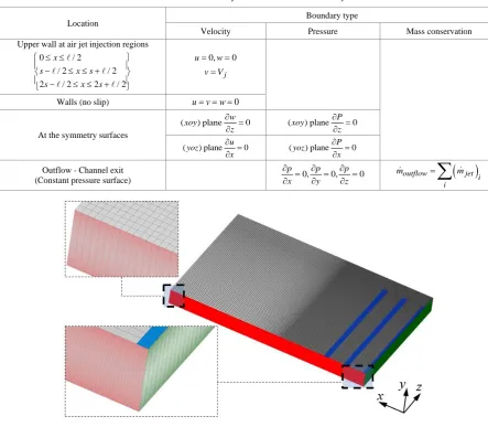
at the slot exit is taken to be 1.0-percent in numerical analysis. At the channel outlet, the pressure is specified to be atmospheric. In addition, the mass flow rate at one of the channel exit ports has to be compared with the half of the total flow rate through the injection slots at the upper wall. A deviation of less than 1% is allowed in the computations.

Table 1. Flow boundary conditions for numerical analysis

Location Boundary type

Velocity Pressure Mass conservation Upper wall at air jet injection regions

0 / 2 / 2 / 2 2 / 2 2 / 2

x

s x s

s x s

≤ ≤

 

 _{− ≤ ≤ +} 

 

 _{− ≤ ≤ +} 

 



 

 

0, 0

u= w=

j

v=V Walls (no slip) u= = =v w 0

At the symmetry surfaces

(xoy) plane w 0

z

∂ ₌

∂ ( ) plane 0

P xoy

z

∂ ₌ ∂

(yoz) plane u 0

x

∂ ₌

∂ ( ) plane 0

P yoz

x

∂ ₌ ∂

Outflow - Channel exit

(Constant pressure surface) 0, 0, 0

p p p

x y z

∂ ₌ ∂ ₌ ∂ ₌

∂ ∂ ∂ outflow

( )

jet i

i

m =

∑

m

3.2. Solution Procedure and Mesh Independency

As illustrated in Fig. 1b, the geometrical dimensions of the channel and the reference frame are the same as in experiments. In the analysis, the channel height varies between 12.7 mm and 38.1 mm, and depending upon the slot spacing, s, the injection region of the channel extends from 114.3 mm to 215.9 mm. However, the channel length is kept constant at 1000 mm in the analysis. As shown in Fig. 1b, due to flow symmetry along

(

xoy

)

and

(

yoz

)

planes, one-fourth portion of the channel sized with the arrangement in length

×

height

×

width as 500×(12.7, 25.4, 38.1)×330 mm is considered as the computational domain. To ensure that near wall region, the wall unit;

y

+

=

u y /

_τ

ν

, values are less than or close to unity, the nodes close to the walls are denser than the meshes at the central region of the channel. In addition, enhanced wall-function is considered to capture accurately high values of velocity gradients along the channel surface. Referring to the grid distribution as illustrated in Fig. 4, quadrilateral meshes starting with the size of 1.0×0.1×2.0 mm at both upper and lower walls of the symmetry plane

(

yoz

)

, and ending with 4.0×0.5×5.0 mm-sized meshes at the center of the channel-outlet are used for computations in the prescribed domain. Reynolds Averaged Navier Stokes equations (RANS), Equations (3)-(5), are discretized by the finite volume technique (Versteeg and Malalasekera, 2007). The pressure-correction algorithm SIMPLE is used for pressure-velocity coupling. Convective terms are

discretized by the upwind scheme and the diffuse terms by the centered scheme. The convergence criterion is 10−5for the residuals of all variables. Then the total mass flowrate at the exit of the computational domain is compared with the counterpart value at the inlet of the injection slots. A deviation error of 1-percent or less is considered acceptable for a solution inside the channel.

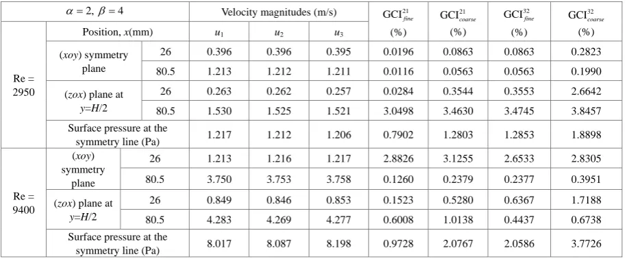
A mesh independency analysis is carried out for two flowrates at Re = 2950, and 9400, at a fixed channel geometry of

α

=2, and

β

=4 . Three cases of mesh density variation with the node arrangement in length× height×width are established as, Case A (fine): 626

×

76

[image:6.595.70.528.473.662.2]

×

165, Case B (medium): 315

×

76

×

110, and Case C (coarse): 221

×

60

×

83. Grid Convergence Index (GCI) is used to show the grid refinement effect on the following parameters: 1. the velocity profiles at (xoy) symmetry plane and at (zox) plane situated at the mid-section of the channel (y = H/2) with locations at x = 26 mm and 80.5 mm are considered. 2. The static pressure distribution along the intersection of the lower wall with the channel symmetry plane

(

xoy

)

. All equations provided by Çelik et al. (2008) are used for calculating the GCI results as given in Table 2. In this table, sub/super-scripts refer to the grid size starting from 1 as fine, 2 as medium, and 3 as coarse. The GCI value could be between 0.0116% and 3.0498% for fine grid evaluations in velocity distribution. Based on the selected grid sizes, the maximum discretization error for fine grid evaluation is calculated to be 1.53

×

3.0498%

=

±0.0466 ms-1 in velocity and 0 078± . Pa in pressure. Due to low GCI and reduced time cost, medium mesh size (Case B) is chosen for the analysis.

Table 2. Estimation of grid convergence index (GCI)

2, 4

α= β= Velocity magnitudes (m/s) 21

GCIfine

(%)

21

GCIcoarse

(%)

32

GCIfine

(%)

32

GCIcoarse

(%)

Re = 2950

Position, x(mm) u1 u2 u3

(xoy) symmetry plane

26 0.396 0.396 0.395 0.0196 0.0863 0.0863 0.2823 80.5 1.213 1.212 1.211 0.0116 0.0563 0.0563 0.1990

(zox) plane at

y=H/2

26 0.263 0.262 0.257 0.0284 0.3544 0.3553 2.6642 80.5 1.530 1.525 1.521 3.0498 3.4630 3.4745 3.8457 Surface pressure at the

symmetry line (Pa) 1.217 1.212 1.206 0.7902 1.2803 1.2853 1.8898

Re = 9400

(xoy) symmetry

plane

26 1.213 1.216 1.217 2.8826 3.1255 2.6533 2.8305 80.5 3.750 3.753 3.758 0.1260 0.2379 0.2377 0.3951

(zox) plane at

y=H/2

26 0.849 0.846 0.853 0.1523 0.5280 0.6367 1.7188 80.5 4.283 4.269 4.277 0.6008 1.0138 0.4437 0.6738 Surface pressure at the

4. Results and Discussions

4.1. Free Jet Measurements

Hot wire measurements were conducted in the free jet in the absence of a target impingement surface in order to validate the quality of the flow. The fluctuating component of the velocity (the Root Mean Square (RMS) turbulence)

( )

' '

v v

was determined by

( )

(

)

2

' '

1

1

N

i i

v v

v

v

N

=





=



_

−



_



∑



(6)

in which

v

indicates the mean velocity and computed as,

1

1

N

i i

v

v

N

₌

=

∑

(7)

where

v

_i and

N

are the jet velocity of each sample and the number of samples respectively. For the slot exit measurements, the hot wire probe was located at the centerline of the slot exit (

y

_j

=

0

) and held parallel to the slot surface. Traverses were taken to determine the jet exit velocity and turbulence profiles.

[image:7.595.320.521.80.213.2]

Fig. 5 represents the RMS turbulence intensity variations for two different Reynolds numbers of 2950 and 10500. It has to be noted that at

2

≤

y /



≤

4

, the jet still has the significant core flow and except the region very close to impingement surface, the characteristics of the approaching jet flow will remain the same in the presence of the target surface and the sidewalls. As shown in Fig. 5, the turbulence intensity at the centerline increases as the Reynolds number increases and roughly varies in the range between 0.95% and 1.08%.

Figure 5. Measuring the free jet centerline RMS turbulence intensity at

the slot exit

4.2. Description of the Flow Field and Channel Pressure Distribution

In order to better understand the behavior of the flow patterns within the channel, we represent Fig. 6, the streamlines related to the mean flow field in the symmetry plane for Re=10500, spacing ratio of

s

/



=

3

,and at different height ratios of

α

. As can be seen from Fig. 6a, typically two circulation zones appear between the adjacent slots and an additional one in a region between the final slot and the channel upper wall. Due to flow accumulation, the relative size of the circulation zone gradually decreases as the fluid advances in the channel. Increase in height ratio causes an increase in relative height of the flow reversal region. In fact, the circulation zone between the two adjacent slots splits into two regions dominated by two vortices of opposite circulation. As shown in Figs. 6b and 6c, the primary circulation being in front of the upstream jet delimits the spread of this jet. Similarly, the secondary flow affects the blowing direction of the downstream jet and deteriorates free jet characteristics. The jet interaction and the overall dynamic behavior of the flow may be better explained by pressure measurements as illustrated in Fig. 7.

(a)

α

=

1

(b)

α

=2

(c)

α

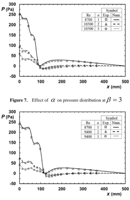
=₃

[image:7.595.140.460.539.734.2]

Figure 7. Effect of

α

on pressure distribution at

β

=

3

Figure 8. Effect of

α

on pressure distribution at

β

=

4

In this figure, due to flow symmetry, half of the pressure data for Re = 8700 and 10500 at slot spacing ratio of

β

=

3

are provided. For the height ratio of

α

=

1

, a steep change in pressure distribution with the occurrence of humps at two locations in downstream direction approximately

extends to the end of the injection section. The location of these humps being at

x

/



=

2.52

and 5.35 corresponds to a region that is covered by the respective slot jets. The pressure assumes a minimum value after the termination of the injection section (x_min/=7.4). Then the increase of pressure in downstream direction signifies the existence of a re-circulatory flow in this region of the channel. Appearance of two vortices at high values of height ratio,

2

α

≥

, causes momentum loss in the approaching jet, and the pressure on the stagnation line is reduced. Hence, for

2

α

≥

, the steep nature of pressure variation disappears. As in Fig. 7, even though the injection velocity for Re = 10500 at

α

=

2

is greater than the case for

α

=

1

, the pressure assumes less values in the injection section. These results are in harmony with the flow behavior as illustrated by the streamlines. Although the pressure distribution in a region after the injection section exhibits an adverse pressure gradient, the location of minimum pressure is not altered for a fixed slot spacing. The pressure measurement data together with the numerical analysis conducted at spacing ratio of

β

=

4

and at height ratios of

1, 2 and 3

α

=

are shown in Fig. 8. No appreciable change in general features of the pressure distribution occurs for

β

=

4

. However, the existence of secondary humps at Re = 8700 in Fig. 8 becomes more distinct for

1

α

=

and these humps move to the right in parallel to the slot-jet movement. In accord with the increase of size of the injection section, the location of the minimum pressure also moves downstream direction for

β

=

4

and occurs at

min

/

9.9

x



=

in Fig. 8. As

α

increases, the pressure assumes lower values in the injection section for

β

=

4

which is considered as a typical flow behavior for all

β

−

values.

(a) β = 2

(b) β = 3

(c) β = 4

Figure 9. Airflow patterns on (xoy) symmetry plane of the channel: effect of

β

and the disappearance of the secondary vorticity at α=2and

[image:8.595.60.284.77.420.2] [image:8.595.142.458.519.714.2]

Fig. 9 represents the streamlines of the flow where the channel height ratio is taken to be

α

=

2

and the spacing ratio

β

assumes values of 2, 3, and 4 at a specified Reynolds number of Re=2950. As in Fig. 9, increase in spacing ratio causes an increase in the size of the primary vorticity. Even though the size increase in vorticity creates some additional resistance to the flow momentum, modifications in flow structure is not sufficient to cause drastic change in pressure drop.

4.3. The Pressure Drop Coefficient

The pressure drop of the injection section is defined as the pressure difference between the stagnation line and the line where injection terminates (∆ =p p(0)−p L( i/ 2)). Owing to the occurrence of highly circulatory flow, the pressure drop in this region of the channel is incomparably higher than the pressure drop of the non-injection section. As an engineering approximation, it can be stated that the frictional characteristics of the channel is basically governed by injection section pressure drop coefficient defined as following,

2

/ 2

p f

V

ρ ∆

= ₍₈₎

Table 3 provides both numerical and experimental data of the pressure drop (

∆

p

) of the injection section for the channel geometric parameters of

1

≤ ≤

α

3

, 2≤ ≤

β

4 and the flow Reynolds number between 1500 and 10500. In determining the scatter of the data, the deviation between the numerical and experimental results for the same geometry and the flowrate is defined as following,

(

1 num/ exp

)

100%

dev= − ∆p ∆p × (9) Hence, the results show that numerical data represent the experimentally evaluated f values within a deviation band covering a range between -16.4% and 3.4%. In

conventional duct flows, the major contribution to the pressure drop is due to high shearing forces that depend on the flow Reynolds number. In the present case, however, the resistance against the fluid motion is essentially caused by vortices. The loss of momentum in the approaching jet due to mixing and constructing a circulatory zone yields pressure loss in air. In fact, careful observation of data in Table 3 describes a trend whereby no appreciable change in

−

f coefficient takes place as the Reynolds number varies when

α

is kept constant.

Meantime, at the same values of

α

and Re, the stagnation pressure (

x

=

0

) is observed to decrease by increasing the jet-to-jet spacing. However, no discernible effect of

β

on f -factor is recorded at a prescribed values of

α

and Reynolds number. For instance, referring to the experimental results in Table 3 for

α

=

1

, and Re = 8700, the

f

-factor typically changes by 7-percent by increasing the spacing parameter,

β

, from 3 to 4. Shariatmadar et al. (2016) also observed similar experimental trends and concluded that the flow characteristics were essentially unaffected by the variation of jet-to-jet spacing within the experimental limits studied. Moreover, referring to data in Table 3, the effect of

β

on

f

-factor at different

α

values is also negligibly small. Accordingly, the least squares linear regression analysis applied to data in Table 3, and the following correlation is recommended for the pressure drop coefficient,

1.75 11.84

α

−

=

f (10)

in which

1

≤ ≤

α

3

, 2≤ ≤

β

4 and

[image:10.595.73.526.89.617.2]

Table 3. Numerical and experimental results for pressure drop coefficient Channel geometry

(mm)

Pressure data (Pa) (Numerical)

Pressure data (Pa) (Experimental)

H/

ℓ s/ℓ Re

Vj

(m/s) Li/2 H Li/2H p(0) p(Li/2) Δp f p(0)

P

(Li/2)

Δp f

1 2

5500 3.28 57.15 12.7 4.50 109.62 22.73 86.89 13.42 9000 5.37 57.15 12.7 4.50 284.74 56.64 228.10 13.14

3

5760 3.43 82.55 12.7 6.50 114.77 23.59 91.17 12.87 6900 4.11 82.55 12.7 6.50 163.17 32.16 131.01 12.88

8700 5.19 82.55 12.7 6.50 256.68 47.08 209.60 12.93 253 73 180 11.1 10500 6.26 82.55 12.7 6.50 367.34 70.66 296.68 12.58

4

1500 0.89 107.95 12.7 8.50 7.35 2.4 4.95 10.38 4800 2.86 107.95 12.7 8.50 77.68 16.83 60.85 12.36 75.33 21.3 54.03 10.97 5900 3.52 107.95 12.7 8.50 116.19 23.84 92.34 12.38

8260 4.92 107.95 12.7 8.50 222.69 41.92 180.76 12.40 221.65 49.86 171.79 11.79 8700 5.19 107.95 12.7 8.50 245.89 44.21 201.68 12.49 240.69 46.05 194.64 12.05

2 2

2950 1.76 57.15 25.4 2.25 8.40 1.85 6.55 3.51 5500 3.28 57.15 25.4 2.25 28.47 5.38 23.09 3.57 9000 5.37 57.15 25.4 2.25 75.49 13.06 62.44 3.60

3

1620 0.96 82.55 25.4 3.25 2.53 0.65 1.88 3.39

2400 1.43 82.55 25.4 3.25 5.63 1.7 3.93 3.19 2950 1.76 82.55 25.4 3.25 8.13 1.68 6.44 3.46

3630 2.16 82.55 25.4 3.25 12.10 2.34 9.76 3.48 5500 3.28 82.55 25.4 3.25 27.31 4.75 22.56 3.48 6900 4.11 82.55 25.4 3.25 42.48 7.08 35.40 3.48 8350 4.97 82.55 25.4 3.25 61.77 10.02 51.74 3.48

10500 6.26 82.55 25.4 3.25 98.33 15.00 83.33 3.53 96.33 19 77.33 3.28

4

2950 1.76 107.95 25.4 4.25 7.82 1.68 6.14 3.29 5560 3.31 107.95 25.4 4.25 26.59 4.77 21.82 3.31 8350 4.98 107.95 25.4 4.25 59.10 9.77 49.33 3.30

9400 5.61 107.95 25.4 4.25 74.71 12.09 62.62 3.31 71.34 18.1 53.24 2.81

3 2

5500 3.28 57.15 38.1 1.50 15.86 3.93 11.93 1.84 9000 5.37 57.15 38.1 1.50 42.23 10.00 32.23 1.86

3

6640 3.96 82.55 38.1 2.17 22.32 3.89 18.43 1.95

8866 5.29 82.55 38.1 2.17 39.35 7.31 32.04 1.90 41.43 10.1 31.33 1.86 10500 6.29 82.55 38.1 2.17 56.37 9.35 47.02 1.97 59.99 11.3 48.69 2.04

4

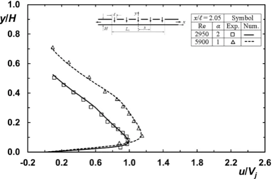
Figure 10. Longitudinal velocity profiles on (xoy) symmetry plane at β =4: comparisons between experimental and numerical results at

/=2.05

x .

4.4. Mean Velocity Distributions

Together with the numerically determined velocity distributions, the mainstream velocity measurements along the channel for

α

=

1

, 2 and at respective Reynolds numbers of 5900 and 2950 are illustrated in Fig. 10. In this figure, to study the effect of the channel height on velocity profile, the slot spacing is kept constant at

β

=

4

. In measuring the mean velocity distribution in the channel, however, the stream-wise location was selected as

/

2.05

x



=

to avoid any contamination due to velocity component in the normal direction,

v

, occurring at very small values of

x

/



( Ashforth-Frost et al., 1997; Zhe and Modi, 2001). Since the Reynolds number for

α

=

1

is taken to be higher than the case of

α

=

2

, higher velocities are expected in the channel. In fact, the maximum channel velocity for

α

=

1

is measured at

/

0.12

y H

≈

and is about 115-percent of the averaged velocity at the slot exit. In case of

α

=

2

, however, the corresponding values for the location and magnitude of the maximum velocity respectively are

y H

/

≈

0.08

, and 96-percent of the slot-jet averaged velocity. Similar data are also reported by Ashforth-Frost et al., (1997) who stated that the maximum velocity for geometric conditions of

H

/



=

4

,

1

<

x

/



≤

3

and at Re=20, 000 prevails over a range 0.015≤ y H/ ≤0.063 with a magnitude of 98-percent of the slot-jet exit velocity. Therefore, the flow characteristics in the neighborhood of stagnation line for

α

=

2

in Fig. 10 resembles a single jet flow, and the growth of the flow reversal region is in direct proportions with the channel height ratio. As the height ratio increases, the relative height of the flow reversal region also increases. A reduction in height ratio and increase in Reynolds number decrease the size of the first re-circulatory zone and its extent in downstream region.

5. Summary and Conclusions

[image:11.595.158.440.80.264.2]

result on the flow behavior is noticed.

The presence of adverse pressure gradient in the area preceding the end of the injection section is well predicted by the numerical simulations, and the complexity of the flow in the separation region is identified. The pressure drop of the injection section,

∆

p

is the dominant parameter in computing the total pressure drop of the channel, and the effect of both geometric and flow conditions on

∆

p

is analyzed. Within the range of flowrates studied, the channel height essentially alters the flow characteristics, and the pressure drop is a strong function of

α

. Hence, the results for the pressure drop coefficient are correlated by using the least square curve fitting technique with a correlation coefficient of 0.99. The good predictions of the realizable k−ε model are also observed in horizontal velocity component measured at the symmetry surface of the channel at x/=2.05.

Nomenclature

A Cross-sectional area [m2]

dh Hydraulic diameter of the injection slot [m]

dev Percent deviation between numerical and experimental results [-]

E Measured voltage difference [mV] f Pressure drop factor [-]

H Channel height [m]

k Kinetic energy of turbulence [m2s-2] L Channel length [m]

Li Length of the injection region [m]

ℓ Slot width (see Fig. 1) [m] p Pressure [Pa]

Re Reynolds number,

Re

ρ

V d

j h

µ

=

[-]

s Slot spacing [m] T Temperature [oC] Ti Turbulent intensity [-] Vj Slot-jet average velocity [ms-1]

W Channel width [m] w Slot length [m]

i j

u u

Reynolds stress component [m2s-2]

u, v, w Velocity components [ms-1] y+ Wall unit,

y

y

τ

w

/

ρ

ν

+

₌

[-] x, y, z Cartesian axis directions

Greek letters

ij

δ

Kronecker symbol

ε

Turbulence energy dissipation rate [m2s-3]

µ

Dynamic viscosity [Pa.s]

ν

Kinematic viscosity [m2s-1]

ϑ

Volume flow rate [m3s-1]

ρ

Air density [kgm-3]

Subscripts

cr Corrected

i, j,k

Vector directions in x, y, z

m Mean value

ref

_Reference

s

Slot

t

Turbulent

∞

Surroundings

Superscripts

Time average

' Fluctuations in velocity

Acknowledgements

The authors would like to acknowledge the financial assistance of Dokuz Eylül University Scientific Research Foundation.

REFERENCES

Afroz, Farhana, Sharif, M.A.R., 2013. Numerical study of [1]

heat transfer from an isothermally heated flat surface due to turbulent twin oblique confined slot-jet impingement. Int. J. of Thermal Sciences 74, 1-13.

ANSYS Inc., 2016. ANSYS FLUENT 17.0 Theory Guide. [2]

Ashforth-Frost, S., Jambunathan, K., Whitney, C. F., 1997. [3]

Velocity and turbulence characteristics of a semi-confined orthogonally impinging slot jet. Exp. Therm. Fluid Sci. 14, 60-67.

Attalla, M., Maghrabie, Hussein M., Qayyum, Abdul, [4]

Al-Hasnawi, Adnan G., Specht, E. 2017. Influence of the nozzle shape on heat transfer uniformity for in-line array of impinging air jets. Applied Thermal Engineering 120, 160-169.

Caliskan, S., Baskaya, S., Calisir, T., 2014. Experimental [5]

and numerical investigation of geometry effects on multiple impinging air jets. Int. J. Heat and Mass Transfer 75, 685-703.

Christensen, K. T., 2001. Experimental investigation of [6]

acceleration and velocity fields in turbulent channel flow. Ph. D. Thesis, University of Illinois at Urbana-Champaign.

Chue, S.H., 1975. Pressure Probes for Fluid Measurement. [7]

Prog. Aerospace Sci., 16, 147-223.

Road, P.E., 2008. Procedure for Estimation and Reporting of Uncertainty Due to Discretization in CFD Applications. ASME J. Fluids Eng 130, 1-4.

Davis, P.L., Renekimer, A.T., Uddin, M., 2012. A [9]

comparison of RANS-based turbulence modeling for flow over a wall mounted square cylinder. 20th Annual Conference of CFD Society of Canada, Canmore, 9-12.

Ebadian, M. A., Lin, C. X., 2011. A Review of [10]

High-Heat-Flux Heat Removal Technologies. Journal of Heat Transfer 133, 110801-11.

Forouzanmehr, M. Shariatmadar, H. Kowsary, F. Ashjaee, [11]

M., 2015. Achieving Heat Flux Uniformity Using an Optimal Arrangement of Impinging Jet Arrays. J. Heat Transfer 137, Transactions of ASME, 061002(1-8).

Gao, X., 2003. Experimental investigation of the heat [12]

transfer characteristics of confined impinging slot jets. Experimental Heat Transfer 16,1-18.

Han, B, Goldstein, R.J., 2006. Jet Impingement Heat [13]

Transfer in Gas Turbine Systems. Annals New York Academy of Sciences, 147-161.

Huber, A.M., Viskanta, R., 1994. Effect of jet-jet spacing on [14]

convective heat transfer to confined, impinging arrays of axisymmetric air jets. Int. J. Heat and Mass Transfer 37, 2859-2869.

Jorgensen, F. E., 2005. How to measure turbulence with [15]

hot-wire anemometers – a practical guide. Dantec Dynamics publication.

Ozmen, Y., 2011. Confined impinging twin air jets at high [16]

Reynolds numbers. Experimental Thermal and Fluid Science 35, 335-363.

Pope, S.B., 2013. Turbulent flows. Cambridge University [17]

Press, Cambridge.

San, J.Y, Lai, M.D., 2001. Optimum jet-to-jet spacing of [18]

heat transfer for staggered arrays of impinging air jets. Int. J. Heat and Mass Transfer 44, 3997-4007.

Shariatmadar, H, Karimi, M.A., Ashjaee M., 2015. Heat [19]

transfer characteristics of laminar slot jet arrays impinging on a constant target surface temperature. Applied Thermal Engineering 76, 252-276.

Shariatmadar, H., Mousavian, S., Sadoughi, M., Ashjaee, M., [20]

2016. Experimental and numerical study on heat transfer characteristics of various geometrical arrangement of impinging jet arrays. Int. J. of Thermal Sciences 102, 26-38.

Slayzak, S. J., Viskanta, R., Incropera, F. P., 1994. Effects of [21]

interaction between adjacent free surface planar jets on local heat transfer from the impingement surface. Int. J. Heat and Mass Transfer 37, 269-282.

Thielen, L., Jonker, H.J.J., Hanjalic’ K., 2003. Symmetry [22]

breaking of flow and heat transfer in multiple impinging jets. Int. J. of Heat and Fluid Flow 24, 444-453.

Versteeg, H.K., Malalasekera, W., 2007. An Introduction to [23]

Computational Fluid Dynamics – The Finite Volume Method, 2nd ed., Prentice Hall.

Yong, S., Jing-zhou, Z., Gong-nan, X. 2015. Convective [24]

heat transfer for multiple rows of impinging air jets with

small jet-to-jet spacing in a semi-confined channel. Int. J. Heat and Mass Transfer 86, 832-842.

Zhe, J., Modi, V., 2001. Near wall measurements for a [25]

turbulent impinging slot jet. J. Fluids Eng. 123, 112-120.

Zuckerman, N., Lior, N., 2005. Impingement Heat Transfer: [26]