The WSN prediction algorithm of real flow based on ARMA model and wavelet transform

Journal of Chemical and Pharmaceutical Research, 2015, 7(3):1025-1030

Research Article

_{CODEN(USA) : JCPRC5}ISSN : 0975-7384

The WSN prediction algorithm of real flow based on ARMA model and

wavelet transform

Guobin Chen and Ting Xie

Rongzhi College, Chongqing Technology and Business University, Chongqing, China

_____________________________________________________________________________________________

ABSTRACT

To improve the prediction accuracy of real flow in wireless network, a new prediction algorithm, state prediction algorithm was proposed basing on ARMA model and Wavelet Transform(SPWA). In this algorithm, first defined distribution character and theoretical foundation of ARMA model, then yielded higher real flow prediction accuracy basing combined predictions of ARMA and wavelet transform. at least, simulations were conducted to study the key factor of algorithm through OPNET and MATLAB. The results show that, comparing to FARIMA model and MF-FIR model, SPWA has better suitability.

Key words: Prediction accuracy; ARMA ; Wavelet; character

_____________________________________________________________________________________________

INTRODUCTION

Wireless sensor network(WSN) grows rapidly from its birth[1-5]. Meanwhile, network jam is more and more concerned because it thresholds the quality of WSN. Some researchers proposed some solutions to eliminate the jam, CODA[6], fusion[7] suggested to control the jam by adjusting the network knots and flow. These two are concerning how to do it during the jam, however, if the jam can be forecasted and then erased before it happened, that will be effectively and efficiently improve the wireless network quality. So how to control real flow and then predict the flow state becomes the key issue. there are some classic network prediction methods like AR, ARMA and FARIMA. Other models such as wavelets transform and chaos model also introduced to real flow prediction. Wei Shan and his colleagues [8] improved ARMA model with super linear convergence of variable metric method and proposed real flow prediction methods based on autocorrelation coefficients and partial autocorrelation coefficients tailing methods. Based on optimized IPSO, Yang Song et al., [9] prolonged searching time of the initial stage and final stage of the iteration to balance entire searching and local searching, and then to optimize model parameters to construct a chaos supporting vector machine model. Hsianghsi Wen et al., studied an optimized sample online fuzzy predicting method via least squares support vector machine and fuzzy LSSVM training, also they studied characters of real flow over time and long period [10]. To improve the high risk Dandan Li et al., successfully improved the prediction accuracy by constructing the Back Propagation network value method through combined wavelet and ant colony algorithm towards traditional predicting method high risk on training data [11]. Chao Li et al., improved logistic model with cosine function, and then depicted state evolution and the chaotic character of real flow using nonlinear time sequence analysis and logistic model [12]. Ting Lei et al., introduced wavelet decomposed the flow time sequence and yielded wavelet transform scaling coefficient sequence and wavelet coefficient sequence, and then taking coefficient sequence as well as original flow time sequence as input and output for the model to construct an artificial neural network to train [13]. Meiying Ye et al., constructed a online fuzzy least squares support vector for real-time updating predicting accuracy but which also effected by time scale [14].

part shows the characters of ARMA model, in the second part shows the judgement foundation of the ARMA and constructs predicting algorithm, in the third part runs simulating on OPNET and MATLAB, and finally a conclusion.

1. ARMA Model

ARMA is known as its high predicting accuracy, realtime and effectiveness. In wireless sensor, a normal flow sequence is: W1,W2,…Wt, can be written as:

t q j j t j p i i t

t

W

a

a

W

=

∑

−

∑

+

= −

=1 − 1

1

ρ

τ

(1)

where

a

_t

∈

N

(

0

,

σ

_a2

)

,τi, ρi are coefficients，at is distract. Eq.(1) presents a p order autoregressive moving average model over m order, can be written as ARMA(p,q), in which p and q are the order indicators of AR and MA respectively. τi(i=1,2,…, p) and ρi (j=1,2,…, q) are model parameters for each part. Here expectation of Wt for E(Wt) is:

∑

∑

= − = −

−

=

m j j t j n i i t t

t

W

a

W

E

1 1

)

(

τ

ρ

(2)

E(Wt) is effected by Wt-i and at-j. Define after moving operator B, so BWt=Wt-1 can be rewritten as:

t t p p t

W

B

B

B

W

=

(

τ

−

τ

−

−

τ

)

+

α

2 2

1

L

(3)

so q order moving average date can be represented as:

t q q

t

B

B

B

W

=

(

ρ

₁

−

ρ

₂ 2

−

_L

−

ρ

)

α

(4)

So the autoregression model of stationary random process ARMA(p,q) is:











−

−

−

=

−

−

−

=

=

q q q P P p t q t p

B

B

B

B

B

B

B

B

B

W

B

ρ

ρ

ρ

ρ

τ

τ

τ

τ

α

ρ

τ

L

L

2 1 2 2 1

1

)

(

1

)

(

)

(

)

(

(5)

take p=2, q=1 for less computing burden, and employ least square to evaluate the model, where the principle of least square is: 2 1 1 0 2 1

)

(

)

(

∑

∑

= = ∧

−

−

=

−

=

N i i i N i i

i

Y

Y

a

a

W

Y

J

(6)

where Yi is the ith observation value of Y, Wi is the ith observation value of W. α0 is intercept and α1 is slope. taking J partial derivative with respect to α0 and α1 can get:













−

−

−

=

∂

∂

−

−

−

=

∂

∂

∑

∑

= = N i i i N i i i

W

a

a

Y

a

J

W

a

a

Y

a

J

1 1 0 1 1 1 0 0

)

(

2

)

(

2

(7)

given the derivative is equal to 0, the equations can be rewritten as:



















−

=

−

−

−

=

∑

∑

∑

∑

∑

∑

∑

= = = = = = = N i N i i i N i N i i i N i N i N i i i i i

W

N

a

Y

N

a

W

N

W

Y

N

Y

W

N

W

1 1 1 0 1 1 2

1 1 1

1

1

1

)

1

(

)

1

)(

1

(

α

(9)

In which the time sequence stable condition is τ1+τ2<1.

2. The predicting algorithm based on combined ARMA and wavelet transform.

Here the specific checking steps. First, take state as St of real flow Wt at the wireless sensor network base station o. Mainly concerned the delay Dt and column length Lt for reducing the sudden of real flow and improving the predicting accuracy. Analyze the current and past real flow state to gain next flow Zt+1 to conduct a reasonable sequence manage. thereafter are the proper predicting algorithm for real flow:

step 1, initial network topology and correlated parameters at the beginning when t=0;

step 2, record the state vector St of real flow Wt at T when t=0, and introduce to ARMA to check if it satisfied the model, if it is then move to step 3, or move to step 7;

step 3, compute the delay Dt+1 and column length Lt+1 of real flow of time t+1:













+

Ω

−

=

−

+

Ω

−

−

=

∑

∑

∞ = + + ∞ = + + + 0 ' 1 0 1 ' 1

)

1

(

)

1

(

)

)

1

((

)

1

(

1

n n k t n n m t

b

n

L

t

b

n

D

λ

λ

(10)

where λ is size of base burden, b is buffer size, and Ωk+n is distribution function of real flow.

step 4, introduce wavelet transform to process the real flow because of the sudden and length, and then combine the predicted results with what yielded in step 2 to minimize the error. decompose delay Dt and column length Lt of Wt with DB2 wavelets can get scale coefficient aj(k) and wavelet coefficient dj(k):









+

+

=

+

+

=

+ + + +

)

1

2

(

)

2

(

)

(

2

)

1

2

(

)

2

(

)

(

2

1 1 1 1

k

d

k

d

k

d

k

a

k

a

k

a

j j j j j j (12)

step 5, employ ARMA to predict wavelet coefficients. evaluate AR(p) parameters τ(1), τ(2), ..., τ(p) and filtering by

the FIR filter

1

( ) 1

( )

p

k

k

A z

τ

k z

−

=

= +

∑

, an approximation process MA(q) can be derived: ρ(1), ρ(2),ρ(3), …, ρ(q),

as well parameters p and q. The predicted wavelet coefficient are also computed through Eq.(6), and then synthesize the delay D’’t+1 and column length L’’t+1 :

1 1 0 1 1 0

''

''

p q

t k t k k t k

k k

p q

t k t k k t k

k k

D

D

u

L

L

u

τ

ρ

τ

ρ

+ − − = = + − − = =



= −

+









_{= −}

₊



∑

∑

∑

∑

(13)







+

=

+

=

+ +

+

+ +

+

'' 1 '

1 1

'' 1 '

1 1

t t

t

t t

t

L

L

L

D

D

D

ϕ

φ

ϕ

φ

(14)

where ϕ and φ are two weighting factors of two different predictions which can be adjusted to gain an optimized result, also define 0≤φ≤1，0≤ϕ≤1，φ+ϕ=1；

step 7, given t=t+1 and then move to step one, and then run the compute again till the end. step 8, runs over.

Fig.1 simulation condition

Fig.2 comparison of delay prediction

Fig.3 comparison of column length prediction

3. Simulation

computing which leads delay in dynamic transformation in real flow. One can figure out that errors by SPWA、 FAEIMA and MF-FIR are 15.34%、 21.57% and 25.34% respectively.

This paper also studied algorithm, especially the effects over variation of key parameters. here taking real flow X and its coefficient function

X

~

S

_α

(

σ

,

β

,

µ

)

, see

exp { [1 sg n( ) tan ( )]} , 1 2

( ) [ ]

2

exp { [1 sg n ( ) ln ]} , 1

j X

j j

E e

j j

α ω

α

πα

µω σω β ω α

ω

µω σω β ω ω α

π

    

− − ≠

Φ = =

− + =

(15)

where α(0< α<2) is characteristic parameter which is used to present burst degree and fractal state of real flow, β

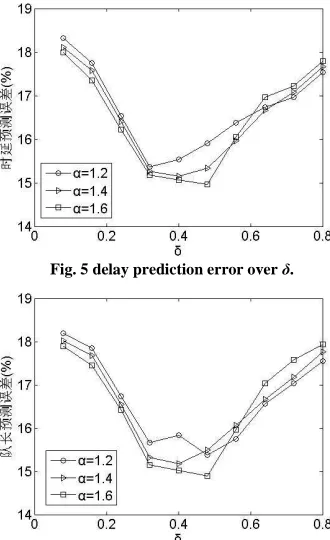
(-1< β <1) is deviation scale parameter, density function shape of real flow is determined by α and β. σ (σ≥0) is deviation scale parameter which represents deviation of distribution, while µ is location parameter which is used to represent average quantity. One can read from Fig. 4 and Fig. 5 that the delay prediction error has a tendency of at first decrease and then increase. When δ is small, bigger α means smaller delay prediction error, while larger delay prediction error when α is growing. This is because bigger α represents bigger real flow. In this paper, ARMA model and wavelet transform are combined for predicting, small δ means wavelet play weights more than ARMA(δ+η=1), wavelet transform is good at erasing emergencies so it shows less prediction error when α is less. When δ is bigger, α play a more important role in low emergency, that’s why smaller α leads smaller prediction error. Also one can read this phenomenon in Fig.4, when δ is small, bigger α leads to small prediction error, and wen

[image:5.595.220.385.362.632.2]

δ is bigger enough, the error hopping contrarily.

Fig. 5 delay prediction error over δ_.

Fig. 5 Column length prediction error over δ_.

CONCLUSION

REFERENCES

[1] Liao H, Lee C, Kedia S P. IET Communications, 2011, 5(7): 914-921.

[2] Yick J, Mukherjee B, Ghosald. IEEE Computer Networks, 2008, 52(12): 2292-2330.

[3] Wu X B, Chen G, Das S K. IEEE Transactions on Parallel and Distributed Systems, 2008, 19(5): 710-720. [4] Chang Y C, Lin Z S, Chen J L..IEEE Transactions on Consumer Electronics, 2006, 52(1): 75-80.

[5] Luo X, Dong M, Huang Y. IEEE Transactions on Computers, 2006, 55(1): 58-70.

[6] Patwari N,Hero A. Using proximity and quantized RSS for sensor localization in wireless net works[C].Proc of the 2nd ACM Int workshop on wireless Sensor Networks and Applications. New York:ACM, 2003:20-29

[7] Li X,Shi H C,Shang Y. A sorted RSSI quantization based algorithm for sensor network localization[C].Pro of

the 11th Int Conf on parallel and Distributed Systems. Los Alamitos,CA:IEEE Computer Society. 2005:557- 563. [8] Shan W, He Q. Acta Electronica Sinica, 2008, 36(12): 2485-2489.

[9] Song Y, Tu X M, Fei M R. Chinese Journal of Scientific Instrument. 2012, 33(4): 757-763. [10] Wen X X, Men X R, Ma Zh Q, Zhang Y Ch. Acta Electronica Sinica, 2012, 40(8): 1609-1616. [11] Li D D, Zhang R T, Wang Ch Ch, Xiao D P. Acta Electronica Sinica,2011, 39(10): 2245-2250. [12] Li Ch, Zhao H, Ge X, Zhang J. Acta Electronica Sinica, 2009, 37(12): 2657-2661.

[13] Lei T, Yu Zh W Computer applications. 2006, 26(3): 526-528.

[14] Ye M Y, Wang X D, Zhang H R., Acta Physica Sinica ,2005,54(6): 2568-2573.

[15] Zhou M Zh, QUan Y Ch, Guo Y, Liu X M, Su Zh L. Journal of system simulation. 2004, 16(2): 306-309. [16] N Sadek, A Khotanzad, T Chen. ATM dynamic bandwidth allocation using FARIMA prediction model[C]. In Proceedings of International Conference on Computer Communications and Networks, 2003: 359-363