Dengue Possibility Forecasting Model using Machine Learning Algorithms

(1)

Dengue Possibility Forecasting Model using Machine Learning

Algorithms

P.Muhilthini

*1

_{, B.S. Meenakshi}

*2

_{, S.L. Lekha}

*3

_{, S.T. Santhanalakshmi}

*4

1,2,3 _{B.E., Department of CSE, Panimalar Engineering College, Chennai, Tamil Nadu, India. Asst.Professor,} 4. _{Department of CSE, Panimalar Engineering College, Chennai, Tamil Nadu, India}

---***---Abstract - Dengue is fast emerging pandemic-prone viral disease, with more than one third of the world’s population at stake. It is also known as break-bone fever. The Aedes mosquitoes, including Aedes albopictus and Aedes aegypti, serve as the main and foremost transmission vector of dengue viruses . In order to curb this problem, it’s necessary to create a predictive system which can minimize the damage and loss in advance. Our dengue incidence prediction model incorporates Gradient Boosting Regression (GBR) algorithm and Mean Square Error (MSE) to measure the performance of the model. Dataset for Dengue gives information about the patients suffering with the dengue disease. The Dataset consist of attribute like temperature, rainfall etc… GBR has the ability to handle heterogeneous data with high levels of predictive power. MSE is directly interpretable in terms of measurements units and so it is a better measure of goodness of fit. A real time adaptive computation software will be developed that could predict the dengue incidences in advance.

Key Words: Pandemic-prone, Dataset, Attribute,

Gradient Boosting Regression (GBR); Mean Square Error (MSE).

1. INTRODUCTION

Understanding the nature of dengue fever is essential to address the spread, outbreak, and prevention of the disease. Dengue fever is common in more than 110 countries, Dengue is a life threatening disease, caused by the mosquito extent in the body of humans and leads to mortality. Dengue fever virus (DENV) is an RNA virus of the family Flaviviridae; genus Flavivirus. Dengue fever is a vector-borne disease, spread by a vector (Aedes mosquito including Aedes albopictus and Aedes aegypti , serve as the main and foremost transmission vector of dengue viruses ) through biting a host (infected human). When a mosquito carrying dengue virus bites a person, the virus enters the skin together with the mosquito's saliva. It binds to and enters white blood cells, and reproduces inside the cells while they move throughout the body. Typically when a mosquito takes a blood meal from an infected person, it takes two weeks of incubation period for the mosquito to be infectious to a healthy person. Each year, nearly 500 million people are infected by this disease and approximately 10,000 to 20,000 die. A vaccine for dengue fever has been approved and is commercially available in many of the countries, but prediction of infectious disease, such as Dengue, is a arduous task and most of the prediction methods are still in their outset The

disease can be transmitted from human to human via infected blood products and through organ donation, but the chance is low and not considered as the major cause of outbreaks. Previous studies prove that temperature, precipitation, and humidity are critical to the mosquito life cycle. Higher temperatures reduce the time required for the virus to replicate and disseminate in the mosquito. Further, studies indicate that both geographical factors and climatic factors contribute to dengue fever outbreak, leading to the concept of landscape epidemiology. This concept emerges from the facts that most vectors, hosts and pathogens are usually associated with the landscape as environmental determinants. Previously there are studies focusing on landscape characters contributing to mosquito-borne diseases. The World Health Organization (WHO) found that urbanization contributes to dengue fever outbreaks. In recent years, increased studies have focused on landscape epidemiology using data mining and machine learning approaches for better disease prediction.

2. PROPOSED SYSTEM

Temperature, rainfall, humidity are the major attributes for the mosquitoes to flourish. But several factors such as population density, political and economic situation affect the distribution of dengue.

It is aimed to quantitatively assess the usefulness of data acquired by various hospitals and health-care units for the early detection and monitoring of Dengue epidemics, both at country and city level at a weekly basis.

Our model adopts Gradient boosting regression algorithm as it supports heterogeneous data types and provides statistical measures with a better predictive power. It incorporated Mean Square Error for improving the levels of performance as it’s a measure of how close a fitted line is to the data points.

3. EXPERIMENTAL METHODOLOGY

(2)

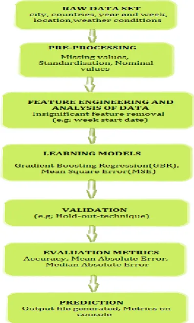
dependencies in the given training dataset and predict number of dengue cases for the given week and year of a country in the test dataset. It collects all the raw dataset (including weather conditions) from the cities for every week and then it involved in the pre-processing step which is done by including the missing values and nominal values. For predicting the data, the Gradient Boosting Regression (GBR) algorithm is used, and in GBR we are using Ensemble Technique. An ensemble is just a collection of predictors which come together (e.g. mean of all predictions) to give a final prediction. Further, Mean Square Error (MSE) gives the difference between the existing and proposed data, (i.e. MSE can represent the difference between the actual observations and the observation values predicted by the model.

Fig -1: Flow diagram for various stages of prediction

4. PRE-PROCESSING:

The dataset contains all the information which the learning model is supposed to learn for making right predictions. The raw data might have a lot of variations in the values of each feature which might lead to incorrect results. Hence the learning process will pre-process the dataset.

The pre-processing techniques include the following;

4.1 Missing Values:

Missing values leads to improper learning, Missing values can be handled in two ways,

i) Removal of Data instances: The data instance which has missing value for any feature was removed. In this way we removed the unreliable data point from the training set but at the same time we have reduced the dataset size from 1456 to 1199.

ii) Filling the missing values: The missing values in the data point were assigned the most frequently occurring value for that feature. We have used the package “preprocessing” and the functionality “Imputer()” from scikits. learn.

We observed that using the second approach (i.e. Imputer) the results were more accurate.

4.2 Standardization:

• There can be huge variation in the values of a feature over the entire dataset. This will make it difficult for the model to learn the data properly. This makes it necessary to standardize the data.

• We have implemented this by removing the mean from the value of each feature and scaling to unit variance. For this purpose we have used the functionality “Standardscalar()” from the pre-processing package.

4.3 Nominal Values:

• The feature “city” in the dataset contains the names of two cities. We need to convert suc values to numerical value. We have implemented the same by using LableEncoder() functionality of the preprocessing package.

5. FEATURE ENGINEERING:

• In any dataset there can be some features which doesn’t have significant effect on the results. Such features need to be identified and can be removed to simplify the data.

• In our dataset we observed that the determining features for number of dengue cases are mainly the year, season of the year and the weather conditions. The week_start_date is redundant attribute. Hence, the feature “week_start_date” was dropped and not considered for analysis of the data.

6. LEARNING MODELS:

6.1 Gradient Boosting Regression:

[image:2.595.57.256.287.618.2]

(3)

and bias. Ensemble helps to reduce these factors (except noise, which is irreducible error). An ensemble is just a collection of predictors which come together (e.g. mean of all predictions) to give a final prediction.

6.2 Mean Square Error:

Mean Square Error(MSE) gives the difference between the existing and proposed data, (i.e. MSE can represent the difference between the actual observations and the observation values predicted by the model. In this context, it is used to determine the extent to which the model fits the data as well as whether removing some explanatory variables is possible without significantly harming the model's predictive ability.

7. VALIDATION:

In our project we are using hold-out technique for validation since the accuracy is found by validation.

7.1 Hold-Out Technique:

The Hold-Out method is the simplest kind of cross validation. The goal of cross validation is to define a dataset to "test" the model in the training phase (i.e., the validation set), in order to limit problems like overfitting, _{give an insight on} how the model will generalize to an independent dataset (i.e., an unknown dataset, for instance from a real problem), etc.

In this method, the mostly large dataset is randomly divided to three subsets:

 Training set is a subset of the dataset used to build predictive models.

 Validation set is a subset of the dataset used to assess the performance of model built in the training phase. It provides a test platform for fine tuning model's parameters and selecting the best-performing model. Not all modeling algorithms need a validation set.

 Test set or unseen examples is a subset of the dataset to assess the likely future performance of a model. If a model fit to the training set much better than it fits the test set, overfitting is probably the cause.

8. EVALUATION METRICS:

The Evaluation process include Accuracy, Mean Absolute Error (MAE), Median Absolute Deviation(MAD).

 Accuracy of the data has been done by using Hold-Out Technique (refer 6.1).

 Mean Absolute Error (MAE) is a measure of difference between two continuous variables. If X and Y are two continuous variable then the difference between X and Y give you the Mean Absolute error(MAE).

 Median Absolute Deviation (MAD) is a measure of statistical dispersion. The Median Absolute Deviation (MAD) is a robust measure of the variability of a univariate sample of quantitative data. It can also refer to the population parameter that is estimated by the MAD calculated from a sample.

9. PREDICTION

[image:3.595.309.561.322.655.2]

In Prediction process, the Output will be generated once if we finish all the above process. As we know, for generating the output, the Dataset is compulsory, here the dataset sample is given below

Fig -2: Data set

10. ALGORITHM:

In our Dengue Possibility Forecasting Model we are mainly using two algorithms and they are;

 Gradient Boosting Regression (BGR)

(4)

The Gradient Boosting Regression(GBR) algorithm is mainly used for predicting the data, and in GBR we are using Ensemble Technique. When we try to predict the target variable using any machine learning technique, the main causes of difference in actual and predicted values are noise, variance, and bias. Ensemble helps to reduce these factors (except noise, which is irreducible error). An ensemble is just a collection of predictors which come together (e.g. mean of all predictions) to give a final prediction.

The reason we use ensembles is that many different predictors trying to predict same target variable will perform a better job than any single predictor alone. Ensembling techniques are further classified into Bagging and Boosting.

 Bagging is a simple ensembling technique in which we build many independent predictors/models and combine them using some model averaging techniques. (e.g. weighted average, majority vote or normal average)

 Boosting is an ensemble technique in which the predictors are not made independently, but sequentially.

One of the most common descriptions of boosted learning is that a group of “weak learners” can be combined to form a “strong learner”.

10.1.1 How Are Weak Learners Combined?

The takeaway is that weak learners are best combined in a way that allows each one to solve a limited section of the problem. Any machine learning routine can be used as a weak learner. Neural nets, support vector machines or any other would work, but the most commonly used weak learner is the decision tree.

10.1.2 Process:

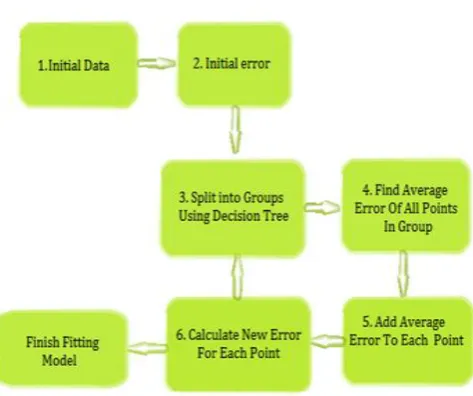
A Regressor attempts to fit a numeric value to something. The something might be fitting the population of a country to GPS coordinates or stock price of a company to monthly sales. The end result of a fitted regression analysis is that you pass in the known features and can predict the unknown output value. Here is the process that boosting regression follows,

 Predict an initial estimate of 0.0

 Use the true values to calculate the error in the initial prediction

 Split the data into groups using the features of the data, with the goal of putting data with similar error into the same group.

 For each group, find the average error

 For every data point in that group, add the average error to the current prediction

 Calculate the new error for each point for the new prediction

[image:4.595.317.554.188.386.2]

 Then repeat the cycle over again starting at step 3 as many times as desired.

Fig-3: Process Of Gradient Boosting Regression (GBR) Algorithm

10.1.3 How Gradient Boosting Works

Gradient boosting involves three elements:

 A loss function to be optimized.

 A weak learner to make predictions.

 An additive model to add weak learners to minimize the loss function.

10.1.4 Improvements to Basic Gradient Boosting:

In this this section we will look at 4 enhancements to basic gradient boosting:

 Tree Constraints

 Shrinkage

 Random sampling

 Penalized Learning

10.2 Mean Square Error:

(5)

harming the model's predictive ability. The smaller the mean Squared Error, the closer you are to finding the line of best fit. The reason minimizing squared error is preferred is because it prevents large errors better.

Mean Squared Error is just Sum Squared Error divided by the number of data points. Since the number of data points is not consistent, optimizing by using MSE will provide means of finding errors with better predictive capability.

[image:5.595.37.288.234.380.2]

11. OUTPUT:

[image:5.595.36.289.279.539.2]

Fig -4: screenshot of dengue prediction possibility

Fig -4.1 screenshot of prediction data from the model

12. CONCLUSIONS

Modeling will show us which features, and which combination of features, will be good predictors of the number of cases. However, it is important to remember that it is not the current weather that determines the number of mosquitoes and thus the number of dengue fever cases. The weeks and months before provide the incubation period for mosquitoes to flourish.

The next post will look into determining the monthly trend (irrespective of the weather features). After that, I will describe methods to use historical weather to predict the current amount of dengue fever cases.

REFERENCES

[1] Shermon S. Mathulamuthu1 , Vijanth S. Asirvadaml , Sarat C.Dass2 , Balvinder S. Gile, Loshini T “Predicting Dengue Incidences Using Cluster Based Regression on Climate Data”. Disease Control Division, Ministry of Health Malaysia (MoH) Universiti Teknologi PETRONAS -2016.

[2] M. U. Kraemer, M. E. Sinka, K. A. Duda, A. Q. Mylne, F. M. Shearer, C. M. Barker, et al., "The global distribution of the arbovirus vectors Aedes aegypti and Ae. albopictus," Elife, vol. 4, p. e08347, 2015.

[3] Loshini T.; Asirvadam, Vijanth S.; Dass, Sarat c.; Gill, Balvinder S. "Predicting localized dengue incidence using ensemble system identification", Computer, Control, Informatics and its Applications (IC3INA), 2015 International Conference on Year: 2015 Pages: 6 - I I.

[4] Duc Ngia Pham, Tarique Aziz, Ali kohan, Syahrul Nellis, Juraina binti abd. Jamil, Jing Jing Khoo, Dickson Lukose, Sazaly bin Abu bakar and Abdul Sattar, " An Efficient Method To Predict Dengue Outbreaks in Kuala Lumpur", Proceeding of the 3"d International Conference on Artificial intelligence and Computer Science (A1CS2015), 12 -13 October 2015, Penang, MALAYSIA. (e-ISBN 978-967-0792-06-4). Organized by http://worldconjerences.net Loshini T.; Asirvadam, Vijanth S.; Dass, Sarat c.; Gill, Balvinder .

[5] Yi-Horng Lai, "Temperature Factor Affecting Dengue Fever Incidence in Southern Taiwan" Asian Journal of Humanities and Social Studies, Vol 02-lssue 05, October 2014.

[6] N. C. Dom, A. A. Hassan, Z. A. Latif, and R. Ismail, "Generating temporal model using climate variables for the prediction of dengue cases in Subang Jaya, Malaysia," Asian Pacific Journal of Tropical Disease, vol. 3, pp. 352-361,2013.

[7] S. Bhatt, P. W. Gething, O. J. Brady, J. P. Messina, A. W. Farlow, C. L. Moyes, et al., "The global distribution and burden of dengue," Nature, vol. 496, pp. 504-507, 2013.

[8] Dom, N., Hassan, A., Latif, Z., & Ismail, R. (2012). Generating temporal model using climate variables for the prediction of dengue cases in Subang Jaya, Malaysia. Asian Pacific Journal of Tropical Disease, 352-361.

[9] Guzman, M. G. et al. Dengue: A continuing global threat. Nature Reviews Microbiology 8, S7–S16 (2010). doi:10.1038/nrmicro2460.

[10] Balmaseda, A. et al. Trends in patterns of dengue transmission over 4 years in a pediatric cohort study in Nicaragua. Journal of Infectious Diseases 201,5–14 (2010). doi:10.1086/648592.