Munich Personal RePEc Archive
Experience and Worker Flows
Gorry, Aspen
UC Santa Cruz
7 July 2010
Experience and Worker Flows
∗
Aspen Gorry
University of California, Santa Cruz
July 7, 2010
Abstract
This paper extends the literature on learning in labor markets by parameterizing the amount of learning that transfers across jobs. Previous models have assumed that learning is either job specific as inJovanovic(1979) or perfectly transferable across jobs as in Gibbons et al. (2005). By allowing some but not all learning to be transferred, this model generates novel predictions of a decline in job finding rates with age and a decline in the variance of wages with experience that are consistent with observed worker outcomes.
∗Please send comments to [email protected]. I thank numerous seminar participants and Fernando
1
Introduction
Learning models account for many important features of labor market behavior. Jovanovic’s
(1979) early work explains broad features of worker turnover behavior: a hump shaped
hazard of separation from a job by tenure and declining separation rates with age. Recent
models use learning to understand wage dispersion, wage growth, and occupational mobility
(for example Moscarini (2005), Farber and Gibbons (1996), Gibbons et al. (2005), and
Papageorgiou (2007)1).
For analytical tractability, the literature on learning focuses on models that make stark
assumptions about the form of learning. On one hand, matching models like Jovanovic
(1979) assume that all learning is specific to a particular job. A worker’s performance on a
particular job provides information only about that job. On the other hand, sorting models
take learning to be about a worker’s ability. In these models, a worker’s performance on
one job generates knowledge about her performance on all other jobs equally. Workers then
use their current belief about their ability to sort themselves into the most profitable job.
These assumptions are stark as workers learn about their ability on a particular job and some
but not all of this information is useful in determining their productivity in other potential
endeavors.
This paper constructs a search model to bridge the gap between these extreme
assump-tions in the literature. The model extends the matching framework to allow agents to learn
not only about their current match, but also allow past learning to be useful in discerning
the quality of their prospective matches when unemployed. This initial screening is similar
toJovanovic (1984), however the amount of information contained in the signal depends on
worker’s past experience. Workers learn rapidly about their ability on a particular match
and some but not all of this learning carries over into future matches. The model
param-eterizes how much learning from one job carries over to understanding how productive the
worker will be in other job opportunities.
1
The model explains how young workers transition from rapid turnover to stable
employ-ment over the life cycle. During the first ten years of labor market experience, workers
transition from high job turnover into stable employment and have rapid wage growth.
About two-thirds of lifetime job turnover and wage growth occurs during these early years
(see Topel and Ward (1992), Flinn (1986)). Initial high turnover manifests itself in both
high job finding and separation rates for young workers. The model is able to explain these
patterns of behavior through learning and experience.
Additionally, the model captures the well known decline in worker turnover with age
(see Clark and Summers (1982)). Past models of turnover have focused on explaining the
decline in job separation rates. However, less focus has been paid to the observed decline
in job finding rates. The model in this paper replicates attractive features of previous
learning models: the decline in unemployment and job separation rates with age and the
rise in wages with labor market experience among other predictions. Allowing experience
to generate differential amounts of learning about current and future jobs generates novel
predictions about the patterns of job finding rates by age and wage dispersion by experience.
The calibrated model generates declining job finding rates with age as experience allows
workers to distinguish between good and bad job offers. For inexperienced workers jobs are
experience goods; they only learn about the quality of the match by trying it out. However,
as workers gain experience jobs become inspection goods. Market experience influences
decisions by unemployed workers about which jobs to accept. As their experience grows,
they reject more bad jobs causing the job finding rate to decline. The past literature on
learning does not generate any prediction on job finding rates. In matching models, learning
is completely job specific so employment forms a renewal process as workers are in an identical
situation each time they become unemployed. In sorting models, although information
transfers between jobs, perfect transfer of information means that workers direct their search
to the job that best fits their abilities. Embedding learning across jobs into a matching
framework generates a mechanism for past experience to alter a workers search behavior and
The calibrated model is then used to generate novel predictions about the volatility of
wages in new jobs. The model predicts wage volatility declines with experience. Intuitively,
more experience from previous jobs generates more information about new matches. This
implies that wages should vary less for workers starting a new job with more past experience.
This new implication from the learning model is confirmed by examining wage data from
the National Longitudinal Survey of Youth 1979 (NLSY79) data.
While there is a large literature that studies wage variation2, few have looked at the wage
variation within job spells3. Learning models have been successful in accounting for these
facts. Farber and Gibbons (1996) consider a baseline model where all learning is public
to provide a theory of observed wage dynamics4. This paper looks at how past experience
influences wage volatility within job spells5. While the cross sectional literature finds that
that wage variation grows as cohorts age (see Rubinstein and Weiss (2006) and Gibbons et
al. (2005)), the result that more past experience reduces individual wage volatility implies
that some of this cross sectional variation is predictable from the individual perspective6.
Related to the literature on learning is an empirical literature that examines the
trans-ferability of human capital across jobs. McCall (1990) explores whether human capital is
job or occupation specific in a similar search model. While my model does not have
occu-pation specific human capital it does capture McCall’s (1990) finding that longer tenure in
the first job implies lower hazard rates in future employment as experience allows workers
to reject poor second matches. Altonji and Shakotko (1987), Topel(1991), and Altonji and
2
For a summary of the literature see Neal and Rosen(2000). Also,Rubinstein and Weiss(2006) nicely summarize the known facts about life cycle wage variation.
3
An exception is the literature on careers in organizations. Baker et al.(1994) summarizes the stylized facts on wages within the firm. While these facts conflict with traditional models of the labor market, enriching standard models of learning have been helpful to explain the data. Gibbons and Waldman(2006) provide a nice summary of the literature and a learning model that can account for many of the features in the data.
4
There is also a small literature that deals with learning, occupational choice, and wages. For examples
see: Miller(1984) andAntonovics and Golan (2008).
5
Jun and Munasinghe (2005) use volatility to try to predict job switching behavior, but do not try to
explain observed volatility.
6
Williams (2005) examine the extent to which wages rise with tenure in a given job rather
than through total job market experience. Learning in my model has both a firm specific
and a general effect. While some experience transfers to allow individuals to better identify
the quality of future matches, workers learn about the quality of their current job at a faster
rate. Although much of wage growth can be accounted for by career experience, there is
still a premium for job tenure. Finally,Mincer and Jovanovic (1982) andBartel and Borjas
(1982) explore the relationship between turnover and wage growth. They find that much of
wage growth is due to general experience while smaller portions can be attributed to firm
experience and mobility choices. These findings are all consistent with model predictions.
The model draws closely from Moscarini(2005) who assumes that jobs are drawn from a
distribution of only two types. Moscarini(2005) andMoscarini(2003) use this trick to embed
Jovanovic’s (1979) model into a general equilibrium framework and explore implications for
the wage distribution. Papageorgiou (2007) extends these models to explore occupational
choices. An empirical literature related to Papageorgiou (2007) on career and job specific
matches seeks to explain the decline in turnover during the life cycle. Neal (1999) presents
a model where workers search for both a career and job specific match. The empirical
implications of career and job matches for job turnover and wages are explored in Pavan
(2007) and Pavan (2006) respectively. My model generates observed declines in job finding
and separation rates without adding the complexity of a second type of career match.
The paper proceeds as follows. Section 2presents the model. Section 3describes how the
parameters of the model are chosen. Section 4presents the results from the calibrated model
about job finding and separation rates, unemployment and wage growth. Section 5 shows
that the model predictions about wage volatility are consistent with data from NLSY79.
2
Model
This section describes the economic environment of an individual making optimal decisions
when faced with uncertain production opportunities (jobs). She searches for production
opportunities and when confronted with one she learns about its quality.
2.1
Production
The infinitely lived worker has preferences given by:
U =
∞
�
t=1
βt−1c
t
There is no storage technology. The worker makes two decisions: when matched with an
opportunity she decides between quitting to search for a new opportunity and continuing to
produce and when unmatched she choose to accept or reject opportunities as she finds them.
Production occurs when a worker is matched with a productive opportunity. In each
period, a match of type µproduces output:
xt=µ+zt
wherezt∼N(0, σ2) is independently and identically distributed noise on the output process.
Therefore,xt ∼N(µ, σ2).
As in Moscarini (2005), the economy is composed of two types of opportunities: µ ∈
{µh, µl}. Let µh > µl so that µh denotes the productivity of a good opportunity and µl
denotes the productivity of a bad one. All production opportunities are drawn independently
from the same distribution where a fraction p0 of them are of type µh.
2.2
Learning
The worker is uncertain about the quality of her current production. She learns about the
current production opportunity and updates her beliefs about the quality of the match using
Bayes’ rule. Second, when an unmatched worker finds a new opportunity she receives a
signal about its quality that depends on her past experience.
While matched, workers observe the output they produce in each period and update
their beliefs. Given the normality of output noise, for any current belief, p, the expected
distribution of output is given by:
ψ(x|p) =p 1
σ√2πe
−12(x−µh
σ )
2
+ (1−p) 1
σ√2πe
−12(x−µl
σ )
2
With probabilitypoutput is drawn from a normal distribution with mean µh and varianceσ,
while with probability 1−pit is drawn from a normal with meanµl and the same variance.
Using this known distribution of output, the worker observers her production and uses
it to update her belief about the probability that she has a good match using Bayes’ rule.
Given any current belief, p, and observed output for a given period, x, the updated belief,
p�, is is formed by conducting a probability ratio test:
f(p, x)≡p� =P rob(µ=µ
h|p, x) =
pe−12(x−σµh)
2
pe−12(x−σµh)
2
+ (1−p)e−12(x−σµl)
2
Here the numerator is proportional to the joint probability of observing output x and the
match being good where the denominator is the total probability of observing output x.
With this updating function, define the inverse function f−1(p�|p) to be the x required
to have posterior p� given priorp. This function is given by:
f−1(p�|p) = σ
2
µh−µl
ln
�
p�(1−p)
(1−p�)p
�
+µh+µl 2
Define the distribution G(p�|p) as the distribution of updates beliefs after observing one
by:
g(p�|p) = ψ(f−1(p�|p)|p)
� � � �
df−1(p�|p)
dp�
� � � �
= ψ(f−1(p�|p)|p)
�
σ2
p�(1−p�)(µh−µl)
�
The process of on the job learning can be generalized beyond the specified output
pro-cess to be some distribution G that depends on the value of the current belief, p, so the
distribution of updated beliefs, p�, is given by G(p�|p). For a general learning process, two
restrictions are made on G. First, G is non-degenerate so that the signal conveys some
information about p. Second, G is restricted so that p is a martingale. This is a natural
restriction since G is used to update an individual’s current beliefs.
When meeting a new match the worker gets an initial signal about the quality of the
match that depends on her past experience. She receives a signal that is equivalent to
observing ατ + 1 observations from the output process. Where τ is months of past work
experience and α ∈ [0,1] determines the fraction of experience that carries over from past jobs into information about new offers. This assumption normalizes the information that a
worker with no experience gets to be equivalent to observing one period of output from the
production process. The normality assumption makes non-integer observations well defined.
Moreover, normality implies that to update beliefs after viewing t observations the worker
only needs to know her prior beliefp, the average value of the observation ¯x, and the number
of observations observedt, not the entire list of observationsx1, x2, . . . , xt. For a worker who
observes t periods of output, the distribution of the average output per period, ¯x, is given
by:
˜
ψ(¯x;p, t) =p σ 1
√
t
√
2πe
−12
�
¯
x−µh
σ
√
t
�2
+ (1−p) σ 1
√
t
√
2πe
−12
�
¯
x−µl
σ
√
t
�2
is computed as:
˜
f(p,x, t¯ ) = pe
−12
�
¯
x−µh
σ √ t �2 pe− 1 2 � ¯
x−µh
σ
√
t
�2
+ (1−p)e−
1 2
�
¯
x−µl
σ
√
t
�2
Again, inverting ˜f gives the value of ¯x needed to generate posterior p�: ˜f−1(p�, p, t) = ¯x.
DefineH(p�|τ) as the distribution of initial beliefs from a new production opportunity. Hence
the p.d.f. of the H distribution,h, is given by:
h(p�|τ) = ˜ψ( ˜f−1(p�, p0, ατ + 1);p0, ατ)
�
σ2
p�(1−p�)(µh−µl)
�
whereαandp0 are parameters. p0 is the prior probability that any new opportunity is good.
The distribution H(p�|τ) can be generalized beyond the specific normality assumptions
described above. In general, forH to provide more information about jobs it must be weakly
increasing inτ in terms of second order stochastic dominance. This means that for τ1 > τ2:
� x
0
H(p�|τ
1)−H(p�|τ2)dp� ≥0 ∀ x∈[0,1]
For higher values of τ workers get more initial information about the quality of a job. This
increasing information for experienced unemployed workers is the novel feature of the model.
A sufficient condition for second order stochastic dominance is that if τ1 > τ2 then H(p�|τ1)
is a mean preserving spread of H(p�|τ
2).
2.3
Wages
Following Jovanovic (1979), the worker’s period payoffs from the production in the model
are given by the expected value of output in each period. Given this output process, the
wage received from a worker is given by:
This wage process is an equilibrium in an environment where there are a continuum of
production opportunities (firms) that have no cost of entering the market. The production
opportunities must make zero expected profits. Under these assumptions any wage process
that pays the average wage along with any matching rate,λ, between workers and production
opportunities can be sustained as an equilibrium outcome7.
2.4
Value Functions
This section defines the value functions for the worker’s general problem. When employed
the worker consumes her wage, ct = w(p), that depends on the probability that her job
is good. The worker can separate from the job for two reasons. First, she could receive
an unfavorable signal about the job quality and decide to quit. Second, with exogenous
probability δ > 0 an employed worker becomes separated from the job in each period. δ
captures reasons for job separations not captured by the endogenous quits that arise from
learning. Possible examples include plant closures or geographic relocation by the worker.
LetV(p, τ) be the value function for an employed worker with beliefpand experienceτ.
The value is written as:
V(p, τ) =w(p) +βδU(τ+ 1) +β(1−δ)
� 1
0
max{U(τ + 1), V(p�, τ + 1)}G(dp�|p) (1)
A worker with beliefp and experience τ gets her expected output w(p). In the next period,
she is separated from her job with probabilityδ, becoming unemployed with experienceτ+1.
With probability 1−δshe is not separated from her job and receives her updated belief from the distribution G. Depending on the realization of her updated belief she can choose to
remain employed with belief p� and experience τ + 1 or quit to become unemployed with
experience τ+ 1.
7
Unemployed workers consume the unemployment value ct =b. b is high enough that if
a worker knows for certain that a job is bad it is optimal to quit and low enough so that if
the worker knows that the job is good that she will work. These assumptions ensure that
the worker’s search problem is non-trivial.
When unemployed, the worker with experienceτ gets an offer from the distribution of jobs
H(p�|τ) with exogenous probability λ. She must choose between remaining unemployed and
becoming employed with beliefp�. If she does not receive a job offer she remains unemployed
with the same experience.
Let U(τ) be the value function for an unemployed worker with experience τ. The value
function is given by:
U(τ) = b+β(1−λ)U(τ) +βλ
� 1
0
max{U(τ), V(p�, τ)}H(dp�|τ) (2)
The final assumption is that experience can only be accumulated for a maximum of T
periods. This assumption allows the model to be computed. It can be justified on two
sepa-rate grounds. First, T can be chosen to be large enough so that workers already have nearly
perfect information about new production opportunities after T periods of past experience.
Second, the finite nature of individual working lives means that workers only accumulate a
finite amount of experience before retirement. The assumption implies that the marginal
value of additional periods of experience is zero once a worker reaches T.
2.5
Model Characterization
The general learning framework described above embeds the the learning models ofJovanovic
(1979) and Gibbons et al. (2005) into a matching framework so the implications of worker
job finding and separation rates can be explored. When α = 0 there is no learning across
jobs and the model is similar to that of Jovanovic (1984) where workers search and get an
initial signal about the quality of a match. In the case ofα = 1, all learning from a particular
opportunity of equal strength to all that they have learned in all past jobs. This embeds the
model of Gibbons et al. (2005) into a matching framework. Different choices of 0≤ α ≤ 1 parameterizes how much information from one opportunity transfers to future ones.
The solution consists of a reservation level of productivity that depends on experience,
¯
p(τ) such that workers will accept jobs or continue working as long as p ≥ p¯(τ) and reject offers or quit otherwise. The general model is rich enough to allow for different
relation-ships between experience, the reservation productivity level, the job finding rate, and wages
that are explored quantitatively in the next sections of the paper. The rest of this section
characterizes these relationships to build intuition about the workings of the model.
First, the reservation productivity level is solved for by setting the value function of a
matched worker with the reservation productivity equal to the value of an unmatched worker
for each level of experience. That is ¯p(τ) solves:
V(¯p(τ), τ) =U(τ) (3)
The sign of ¯p�(τ) is indeterminate.
To see why ¯p(τ) might be decreasing inτ consider the following example. If a worker gets
no extra information about the quality of jobs until she gains t units of experience then she
gets a perfect signal after, there will be a space of experience just before t that the worker
will be willing to accept worse and worse opportunities just to get the payoff from getting t
units of experience. In this case, the option value of experience outweighs the current value
to the worker and can generate decreasing reservation values.
The reservation productivity level will be increasing if the marginal value of information
while employed at the reservation belief is less than the marginal value of information when
unemployed. The reservation value increases when U�(τ + 1) ≤ U�(τ) because extra
expe-rience can only impact a worker when unemployed seeking a new job. This condition can
be interpreted as requiring that the marginal value of experience for unmatched workers is
declining. The direct benefit from the additional unit of experience has to be greater than
This intuition is formalized in the following proposition:
Proposition 1 If U�(τ + 1)≤U�(τ), then p¯�(τ)>0 for all τ ∈ {0,1, . . . , T}.
Proof. See Appendix.
Although, Proposition 1 does not reduce the sign of ¯p�(τ) to restrictions on model
pa-rameters, it provides clear intuition for when the reservation belief will be increasing in
experience. The condition that guarantees ¯p�(τ)>0 is:
Vτ(¯p(τ), τ)≤U�(τ)
Using the results on the worker’s reservation decision above, it is useful to consider
the behavior of the job finding rate. In the model, the job finding rate is determined by
the exogenous rate of matches combined with the workers willingness to accept production
opportunities. The job finding rate as a function of experience, f(τ), is given by:
f(τ) =λ(1−H(¯p(τ),|τ))
Taking the derivative with respect to τ gives:
f�(τ) =−λh(¯p(τ)|τ)¯p�(τ)−λH
τ(¯p(τ),|τ)
whereh(¯p(τ)|τ) is the pdf ofH. For the job finding rate to be decreasing inτ, it is sufficient that ¯p�(τ)≥0 and ¯p(τ)≤ p
0. The first condition guarantees that the first term is negative
and the second condition guarantees that the second term is negative because H(p|τ) is a mean preserving spread around p0. These conditions generate declining job finding rates
early in workers lives where ¯p(τ)≤p0 as workers accept most jobs to gain experience.
The final implications of the model involve the process of the worker’s current belief
p while employed. Given the binary structure of productive opportunities in the model,
the precision of a worker’s beliefs is 1
not necessarily increase over time. However, as the worker gets additional signals about her
current match quality the precision increases on average. This implies that beliefs will change
by a greater degree the further they are from 0.5 as p(1−p) is maximized at that value. While the model in discrete time does not provide a closed form solution for the standard
deviation of G(p�|p), the above intuition shows that the standard deviation is decreasing in
p if p >0.58.
Given the wage process:
w(p) = pµh+ (1−p)µl
the behavior of p can be used to make predictions about the standard deviation of wages.
The novel feature of the model is that a worker with more experience who starts in a new
match will have more information about the quality of that match than a worker with less
experience. In the case where ¯p(τ) > 0.5 and is increasing, the model would predict that
more experience translates to a higher value of p at the start of a new job and a lower
variation in the path of future wages. These implications are quantitively evaluated with
simulations of the model.
3
Calibration
To parameterize the model, assume that there are a large number of workers facing identical
decision problems. Each worker faces a different history of idiosyncratic shocks. Averaging
outcomes across workers, aggregate data are constructed from the model. In computations,
simulated data over a 40 year career is compared to actual worker outcomes. The period
length is one month so that parameters are chosen to match monthly data on job finding
and separation rates in the United States.
To compute the model there are ten parameters that must be chosen: the maximum
amount of experience T, the discount factor β, the job offer rate λ, the expected output
8
In a continuous time analog of the model, the process forpdepends onp(1−p) and the signal to noise ratio of the output process, µh−µl
σ . The termp(1−p)
µh−µl
σ closely approximates the standard deviation of
from a good match µh, the expected output from a bad match µl, the probability that a
match is good p0, the variance of output noise σ, the proportion of experience used for new
matches α, the exogenous separation rate δ, and the value of leisure b.
µh is normalized to one and µl is normalized to zero. Given these normalizations the
evolution of p will be determined by the variance of output noise, σ. The evolution of p
is fully determined by the signal to noise ratio: µh−µl
σ . Because the model period is one
month, β is set to 0.9966 which corresponds to an annual interest rate of 4%. T = 480 to
corresponding to a maximum level of experience of 40 years. This is a reasonable upper
bound as it corresponds to the normal length of work for individuals in the U.S. Increasing
the maximum level of experience has no effect on the results.
The remaining parameters are chosen to match features of the decline in job finding and
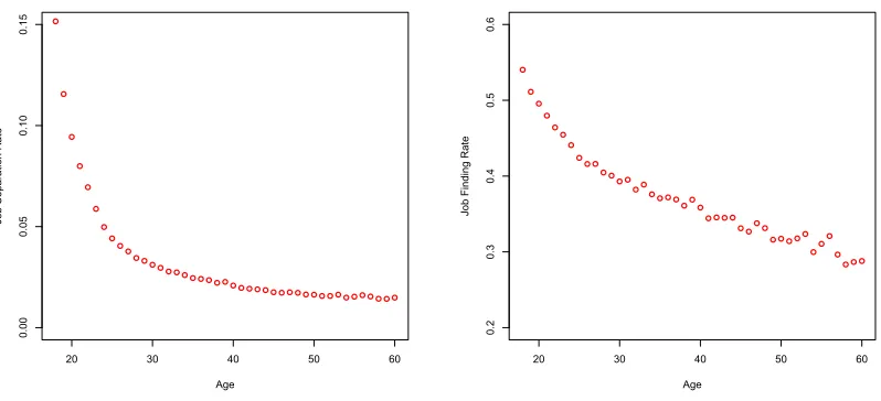
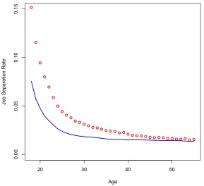
separation rates in the U.S. The left panel ofFigure 1shows the decline in the job separation
rate with age in the U.S. for workers aged 18-579. The separation has a sharp initial decline
from age 18-25 followed by a gradual decline later in life.
The right panel of Figure 1 shows the decline in the job finding rate. Similarly, the job
finding rates fall fastest for the first 8-10 years, but the initial decline is less dramatic than
the separation rate and finding rates continue to decline at a greater rate for the remainder
of the workers’ careers. Notice that while job separation rates fall by about a factor of 10,
the job finding rates only decline by about a factor of 2 over the life cycle. Taken together,
the steeper decline in the separation rate implies that the unemployment rate declines with
age.
λ is chosen to match the worker’s rate of job offers. In the data, 17-year-old workers have
a job finding rate of 0.57. In the model workers with little experience will accept nearly any
productive opportunity that they find. So since workers start at age 18, this provides an
upper bound on the job finding rate. To match this feature of the data, λ is set to 0.6.
9
20 30 40 50 60 0.00 0.05 0.10 0.15 Age Jo b Se p a ra ti o n R a te
20 30 40 50 60
[image:17.612.104.503.111.293.2]0.2 0.3 0.4 0.5 0.6 Age Jo b F in d in g R a te
Figure 1: Monthly job separation rate in left panel and monthly job finding rate in right panel by age for the U.S. economy.
p0 determines the portion of good jobs in the economy. Since a worker with perfect
information about the quality of jobs will only accept good ones,p0 determines the amount
of decline in the job finding rate over the worker’s life. p0 is chosen to match the decline in
the job finding rate found in the data. It is set to 0.7 which allows the model to match the
job finding rate of 0.30 for 57 year old workers in the data.
Next, σ is the amount of output noise. Higher values of σ imply that workers learn
slowly about the quality of their matches. In the limit, σ= 0 implies that workers perfectly
observe the quality of the match with one observation while as σ → ∞ workers have no learning. σ = 4 is chosen to match the shape of the decline in job finding rates. Higher
values ofσ imply that workers learn more slowly. Slower learning implies that it takes longer
to distinguish bad matches, and generates a longer decline in job finding rates. Higher values
of σ imply that the decline in job finding rates is quick and they then level off.
α determines the amount of experience that carries over in learning about new job
op-portunities. It is natural to restrict α to be in [0,1]. α = 0 is analogous to the standard
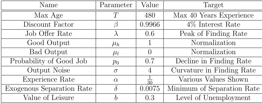
employ-Name Parameter Value Target
Max Age T 480 Max 40 Years Experience Discount Factor β 0.9966 4% Interest Rate
Job Offer Rate λ 0.6 Peak of Finding Rate Good Output µh 1 Normalization
Bad Output µl 0 Normalization
Probability of Good Job p0 0.7 Decline in Finding Rate
Output Noise σ 4 Curvature in Finding Rate Experience Rate α 301 Various Values Shown Exogenous Separation Rate δ 0.0075 Minimum of Separation Rate
[image:18.612.92.516.79.246.2]Value of Leisure b 0.3 Level of Unemployment
Table 1: Calibrated values of the model parameters.
ment is a pure renewal process. α = 1 is the limit where all learning carries over to future
jobs. Higher values of α imply that workers learn faster about future jobs and therefore
have a steeper decline in both job finding and separation rates. Model results for various
values of α are shown. With the model period set to be a month, α= 1
30. This corresponds
to getting one month worth of information about a new job for every two and a half years
of labor market experience. Higher values of α predict a steeper initial decline followed by
less learning later. This parameter is sensitive to the choice of σ. The chosen value of σ
implies that individuals learn quickly by observing output. Surprisingly, very low values of
α generate large changes in the patterns of job finding rates.
δ is the rate of exogenous job separations. An upper bound on the value of δ is lowest
observed monthly job finding probability in the data is 0.014 for 59-year-olds. A lower value
of δ= 0.0075 is chosen.
The final parameter is b. This parameter determines the relative desirability of being
employed in a bad job compared to searching for a new job. Higher values of b make
unemployment more attractive. b= 0.3 is chosen to match the level of unemployment over
a workers lifetime.
≤18 19 20 21 22 23 24 ≥ 25 29.6 24.9 18.8 11.4 8.1 4.8 1.7 0.7
Table 2: Percent of populations first employment spell by age. From Topel and Ward(1992).
4
Simulated Results
This section documents the implications from the calibrated model. The novel feature of
allowing learning to transfer between jobs through work experience is that past experience
now has implications for workers while unemployed through their job search behavior. To
document this, the value functions are computed to generate reservation probabilities for
workers at each experience level. Using these decision rules, employment outcomes are
simulated for individual workers. Monthly employment, job finding rates, job separation
rates, wages, tenure, and total experience are recorded in the simulations. The outcomes for
10,000 simulated workers are computed from the date that workers enter the labor force.
To compare outcomes with labor force data, outcomes by age are constructed by entering
workers into the labor market at the age they get their first full time employment. Topel
and Ward(1992) compute the percentage of workers who enter the labor force at a given age
by assuming that workers enter when they attain their first employment that lasts at least 2
quarters. This measure leaves out workers who take summer jobs and then return to school.
Table 2 replicates their table showing the percentage of workers who enter the labor force
at each age. When constructing the data from the model, all workers in the ≤18 category enter at age 18 and all workers in the ≥25 category enter at age 25.
The remainder of this section compares the simulated data from the calibrated model
with the data.
4.1
Job Finding Rate
The first result is that the calibrated model is able to match the decline in job finding rates
20 30 40 50
0.2
0.3
0.4
0.5
0.6
Age
Jo
b
F
in
d
in
g
R
a
[image:20.612.156.444.109.373.2]te
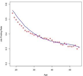
Figure 2: Job finding rate by age. Data: dots; Calibrated Model: Line.
experienced workers are more selective about which jobs they choose to accept. This feature
allows the job finding rate to decline over a worker’s lifetime.
Figure 2 plots the decline in job finding rates from the simulated model against the data.
Simulated job finding rates start out slightly higher and decline to match the rates observed
in the data. The two series are almost identical after age 30. The calibrated model is able
to capture the initial steep decline in job finding rates and continued gradual decline later
in life. No previous models of learning generated any change in job search behavior so their
predicted job finding rate is constant.
To compare the fits of the model with the data a goodness of fit is computed:
F it= 1−
�57
a=18(εa−ε¯)2
�57
20 30 40 50
0.2
0.3
0.4
0.5
0.6
Age
Jo
b
F
in
d
in
g
R
a
te
! = 1
! = 1/12
! = 1/24
! = 1/30
! = 1/48
[image:21.612.158.441.107.373.2]! = 0
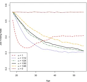
Figure 3: Job finding rate by age for various values of α.
This is similar to anR2 measure, where ε
a is the difference between the model and the data
for age a, ¯εis the average difference,ya is the level of the data for agea, and ¯y is the average
level of the data. The numerator give the sum of squared errors between the data and the
model and the denominator gives the sum of squared deviations in the data. The calibrated
model has a fit of 0.95.
To see how changes in α affect the results of the model, Figure 3 plots the job finding
rate from the calibrated model for different values ofα. Low values of alpha imply a steeper
initial decline in job finding rates as the worker is more quickly able to distinguish between
good and bad jobs. In the cases close to the calibrated value of α = 301 the simulated job finding rates decline throughout the worker’s simulated working life. However, for high
is a large portion of the worker’s life for which the job finding rate is increasing. Recall that
for a worker with perfect information, the job finding rate is determined by the arrival rate
of productive opportunitiesλmultiplied by the fraction of those opportunities that are good
p0. This gives a job finding rate of 0.42 for the current calibration. The initial rapid decline
occurs as some information about the quality of the job initially makes the worker much
pickier about which jobs to accept. Over time better information pushes a greater portion
of jobs above the threshold to increase the job finding rate. The case of α = 481 shows that even small amounts of learning across jobs can have dramatic effects on the predicted
worker search behavior over the life cycle. Finally, the case of α = 0 is shown to be flat.
This corresponds to the Jovanovic (1979) model where no learning transfers across jobs and
workers have a flat job finding rate for their entire life.
4.2
Job Separation Rate
Figure 4 shows the decline in separations for the calibrated model compared with the data.
The model exhibits an initial decline in the separation rate that is steeper than the data,
but is unable to generate the highest levels of separations for young workers. Some of the
high rates are due to workers moving in and out of the labor force for schooling that is not
captured by the model. The decline in job separations happens in the model for two reasons.
First, as in Jovanovic (1979) the job separation rate declines as workers sort themselves
to good jobs which last longer on average than bad jobs. Second, experience allows older
workers to match with better jobs than younger workers reducing the chance of separation
for new jobs acquired later in life.
The fit of the calibrated model is 0.68. Despite not capturing the high level of initial
separations in the data, the model with learning is still able to capture most of the decline
20 30 40 50
0.00
0.05
0.10
0.15
Age
Jo
b
Se
p
a
ra
ti
o
n
R
a
[image:23.612.155.444.111.375.2]te
Figure 4: Job separation rate by age. Data: dots; Calibrated Model: Line.
4.3
Unemployment
It is well known that young workers face higher unemployment rates than prime aged workers.
The model is able to capture this decline in unemployment with age.
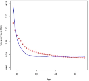
Figure 5 shows the average annual unemployment rate by age. The dots depict the
decline in unemployment found in the data where the solid line depicts the results from the
calibrated model. The data show a steady decline in unemployment with age. Unemployment
declines from about 17% for 18-year-old workers to between 3.5 and 4% for prime aged
workers. The calibrated model captures a similar decline over the life cycle, with 18-year-old
workers experiencing unemployment of 23% and declining to 4.1%. The initial decline in
unemployment is steeper in the calibrated model than in the data reflecting all 18 year old
20 30 40 50
0.00
0.05
0.10
0.15
0.20
0.25
Age
U
n
e
mp
lo
yme
n
t
R
a
[image:24.612.157.444.113.374.2]te
Figure 5: Unemployment rate by age. Data: dots; Calibrated Model: Line.
data is 0.75.
The predicted decline in unemployment from the model can be understood by combining
the results about declining job separation and job finding rates. The decline in job separation
rates drives most of the decline in unemployment while the decline in job finding rates tends
to slightly increase the unemployment rate. However, the decline in separations dominates
as it goes from about 7.5% to 1.3% over the worker’s life while the job finding rates only
decline by about a factor of 2 from about 56% to 30%.
4.4
Wage Growth
Flinn (1986) argues that wage growth and turnover are related for young workers. This
doc-20 30 40 50
0.6
0.7
0.8
0.9
1.0
Age
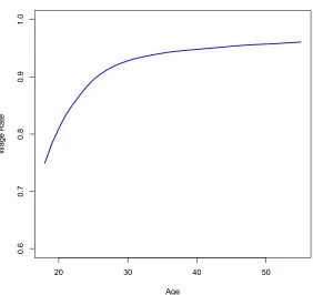
[image:25.612.159.441.106.372.2]Wage Rate
Figure 6: Wages by age in calibrated model.
ument a number of features of wage profiles during worker’s first 10 years of experience.
They document that the first 10 years of the career account for two-thirds of lifetime wage
growth. Job changes explain about one-third of wage growth. Moreover, wages on the job
approximate a random walk. The model qualitatively replicates the behavior of wages over
the life cycle.
Figure 6 shows the average annual wages by age from the model. The pattern of wage
growth from the model is endogenous. The model generates rapid wage growth during the
first 10 years of experience and then levels off. While the model matches the general pattern
of wage growth, it doesn’t generate quite as much wage growth as found in the data where
wages about double over the lifetime. This should be expected as the model generates only
growth from learning by doing or other forms of human capital gained while working. A
model would need to include these other forms of wage growth to fully account for wages
over the life cycle.
5
Wage Volatility
This section quantitatively evaluates the model’s predictions on wage variation using data
on wages and job switching from NLSY79. The novel feature of this model is that workers
who start jobs with more experience have better information about the quality of their new
job. For standard parameterizations, this information means that experienced worker’s on
average start with a higherpand hence their wages should display less variation in subsequent
periods. These predictions are first confirmed using observations simulated from the model
then the same results are documented using data from the NLSY79.
The NLSY79 is a nationally representative longitudinal survey conducted by the Bureau
of Labor Statistics that samples 12,686 individuals who were between the ages of 14 and 22
years old when first surveyed in 1979. The individuals continued to be surveyed every year
until 1994 when the survey switched to every two years. The data are restricted to before
1994 so that appropriate measure of annual wage volatility within jobs can be constructed.
NLSY79 provides a rich set of panel data for tracking worker’s career outcomes. To avoid
miscalculation of past experience, the sample is limited to workers who are 17 years old or
younger at the time of the first interview.
To construct job variables the NLY79 provides a variable for the total number of past
jobs that the respondent has held. In the NLSY a job is defined as a relationship between
an individual employer and the worker. That is changes in position within a firm are not
considered new jobs. If the total number of jobs in year t is greater than in year t−1, then there is a new job observation. For each job observation the wage in each year is given by
the CPS wage10. Finally, experience can be constructed by taking a cumulative sum of the
10
weeks worked in the past year variable. The number of past weeks worked is multiplied by
52 so that results can be presented in terms of years of experience. To compare observed
outcomes from the NLSY79 with the model, 25 years of annual observations are simulated
for the worker’s employment status, past experience, accumulated job number, and wage
from the model. To make the samples comparable, both the simulated and NLSY79 data
are restricted to jobs where workers start with less than 15 years of prior experience.
Each worker’s employment history is broken into jobs that are characterized by a wage for
each year of tenure on the job and the initial experience level when starting the job. Wage
volatility is measured as the absolute deviation from the worker’s expected wage growth
path. The simplest measure of wage volatility is to take the absolute value of the difference
in log wages at each tenure level from the initial wage on the job. However, this measure
does not control for the expected levels of wage growth that occur at different levels of tenure
and experience. To control for this, the wage volatility measure used is:
vt =|log(wt)−log(w0)−w¯et|
vt is the volatility of wages at tenure t on a given job11. wt is the wage observed at tenure
t, w0 is the initial wage observed on the job, and ¯wet is the median log wage deviation
(log(wt)−log(w0)) observed for the two year initial experience group e and tenure levelt12.
By construction the volatility is zero for the initial wage observation (worker’s tenure of
zero). Note that the concept of wage volatility here is at the individual level rather than a
annual data is taken from the simulated model. In the simulated model a worker’s wages change every month based on their updated beliefs. Treating the simulated data the same as the NLSY79 observations should yield similar biases.
11
vt is thetyear measure of volatility, sov3 measures the volatility of wages over a three year increment
from starting the job. Another measure of volatility,v(t) can be defined as the one year volatility for each yeart from the previous years observed wage:
v(t) =|log(wt)−log(wt−1)−w˜¯et|
Where ˜¯wetis the median log wage deviation (log(wt)−log(wt−1)) for the two year initial experience groupe
and tenure levelt. The rest of the analysis focuses on the first year volatility on a job, so these two measures are identical.
12
0 2 4 6 8 10 0.050 0.055 0.060 0.065 0.070 0.075 Years Experience Me d ia n W a g e Vo la ti lit y
0 2 4 6 8 10
[image:28.612.103.502.112.291.2]0.095 0.100 0.105 0.110 0.115 0.120 Years Experience Me d ia n W a g e Vo la ti lit y
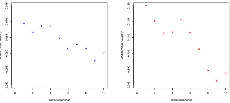
Figure 7: Median wage volatility (v1) by years of past experience. Simulated model in left
panel NLSY79 data in right panel.
cross section across individuals. Higher volatility implies that a given individual experiences
larger changes in her wages on a given job. By subtracting ¯wet the measure of volatility used
in this paper controls for median wage gains in each year of tenure at a particular job and
with experience. While most workers get wage increases from year to year, subtracting of
the expected wage growth at the tenure and experience level means that many workers are
both above and below the expectation.
While the effect of experience on wages has been explored by a large theoretical literature
(SeeNeal and Rosen(2000),Gibbons et al.(2005)), the previous literature has not explored
the impact of experience on individual within job wage volatility. Understanding the
fea-tures of the individual income process is important to explain a wide array of individual
behavior (see Meghir and Pistaferri(2004)). This paper shows that past job experience has
a predictable effect on individual wage volatility. Experience is shown to decrease individual
level uncertainty about wages while cross sectional heterogeneity may increase within group
wage variation. The model is able to account for the individual level declines in volatility.
experience. To explore this prediction, it is sufficient to just look at the first year wage
volatility on each new job,v1. The left panel ofFigure 7plots the median wage volatility for
the first year in each job binned by years of past experience. The model generates a decline
in wage volatility for workers with more past work experience. Note that the model predicts
that for inexperienced workers the one year change in wages will be about 7%. Median
volatility declines to under 6% for workers with 10 years of experience. The right panel of
Figure 7plots the median wage volatility for the first year in each job with experience binned
into yearly groups for the NLSY79 data. Just as in the simulation the data shows a decline
in wage volatility for workers with more past work experience. For inexperienced workers,
the one year change in wages is about 12%. Volatility declines at a steeper rate to under
10% for workers with 10 years of experience. The patterns of volatility with experience are
consistent with those found in the model. Note that there is a scale shift between the two
panels in the figure. Since the magnitudes of wage volatility are higher in the data, the
model does not capture all of the observed wage volatility. However, the similar declines
with experience imply that the model explains a large portion of the interaction between
experience and volatility found in the data.
To more formally assess the model’s predicted effect of experience on wage volatility, the
year one wage volatility measure v1 is regressed on the past experience associated with each
new job event. Quantile regressions are valuable for two reasons. First, they are robust to
the lower bound issues in observed volatility. Second, they provide a more details predictions
about how experience influences volatility at different points in the distribution so that the
model predictions can be more closely compared to the evidence found in the data. This
gives additional feedback about how experience influences workers at different parts of the
volatility distribution. Quantile regressions are run for the 5th, 10th, 25th, 50th, 75th, 90th,
and 95th percentiles13.
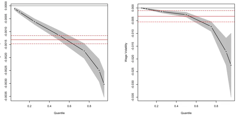
The left panel of Figure 8 shows the results for the OLS regression plotted against the
quantile regression results. The graph shows that both the OLS and median quantile
regres-13
0.2 0.4 0.6 0.8 -0 .0 0 3 5 -0 .0 0 3 0 -0 .0 0 2 5 -0 .0 0 2 0 -0 .0 0 1 5 -0 .0 0 1 0 -0 .0 0 0 5 0.0000 Quantile W a g e Vo la ti lit y
0.2 0.4 0.6 0.8
[image:30.612.110.505.98.291.2]-0 .0 3 5 -0 .0 3 0 -0 .0 2 5 -0 .0 2 0 -0 .0 1 5 -0 .0 1 0 -0 .0 0 5 0.000 Quantile W a g e Vo la ti lit y
Figure 8: Plot of quantile regression of first year wage volatility on past experience with error band. Thin lines gives OLS estimate with dashed error bands. Simulated model in left panel NLSY79 data in right panel.
sion confirm a negative and significant effect on wage volatility. The quantile regressions at
other points in the distribution show that at higher percentiles of the distribution experience
causes larger decreases in wage volatility. The right panel of Figure 8 plots the regression
results of wage volatility on experience from the NLSY79 data. Again, the patterns in the
regressions confirm the model predictions. Both the OLS and median quantile regression
show a significant negative effect of experience on wage volatility. The magnitude of the
decline is between 23 and 32 basis points per year of experience depending on using the
median quantile regression or the standard OLS estimate.
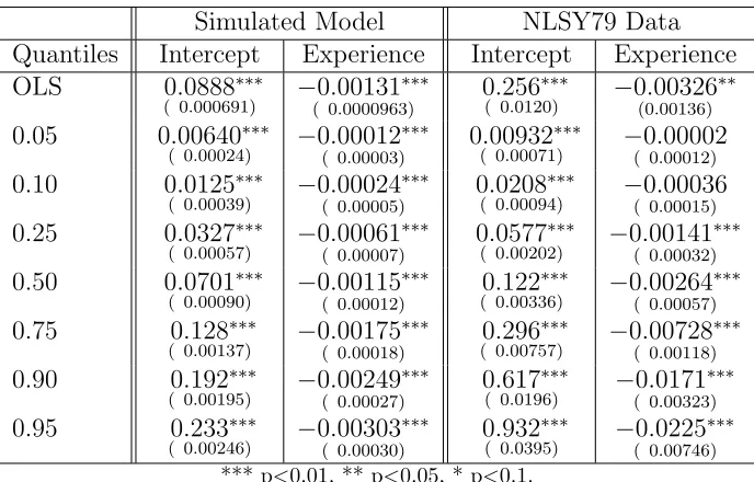
The regression results for both the model and NLSY79 data are presented inTable 3. The
estimated effect for the median and mean in the model is that an extra year of experience
decreases the volatility of wages by about 13 basis points. The coefficient on experience is
negative and significant in all cases except for the 0.05 quantile. This is expected as wage
volatility is close to zero for the low quantiles and hence cannot decrease much further. The
Simulated Model NLSY79 Data Quantiles Intercept Experience Intercept Experience OLS 0.0888∗∗∗
( 0.000691) −0.00131
∗∗∗
( 0.0000963) 0.256
∗∗∗
( 0.0120) −0.00326
∗∗
(0.00136)
0.05 0.00640∗∗∗
( 0.00024) −0.00012
∗∗∗
( 0.00003) 0.00932
∗∗∗
( 0.00071) −( 00..0000200012)
0.10 0.0125∗∗∗
( 0.00039) −0.00024
∗∗∗
( 0.00005) 0
.0208∗∗∗
( 0.00094) −( 00..0003600015)
0.25 0.0327∗∗∗
( 0.00057) −0.00061
∗∗∗
( 0.00007) 0.0577
∗∗∗
( 0.00202) −0.00141
∗∗∗
( 0.00032)
0.50 0.0701∗∗∗
( 0.00090) −0.00115
∗∗∗
( 0.00012) 0.122
∗∗∗
( 0.00336) −0.00264
∗∗∗
( 0.00057)
0.75 0.128∗∗∗
( 0.00137) −0.00175
∗∗∗
( 0.00018) 0.296
∗∗∗
( 0.00757) −0.00728
∗∗∗
( 0.00118)
0.90 0.192∗∗∗
( 0.00195) −0.00249
∗∗∗
( 0.00027) 0.617
∗∗∗
( 0.0196) −0.0171
∗∗∗
( 0.00323)
0.95 0.233∗∗∗
( 0.00246) −0.00303
∗∗∗
( 0.00030) 0
.932∗∗∗
( 0.0395) −0.0225
∗∗∗
( 0.00746)
*** p<0.01, ** p<0.05, * p<0.1.
[image:31.612.134.478.77.297.2]Robust standard errors clustered by individual in parentheses.
Table 3: OLS and quantile regression results for the simulated model and the data.
with higher wage volatility. The results from the NLSY79 data confirm this general pattern.
The OLS estimate indicates that a year of experience decreases volatility by about 33 basis
points while the median decreases by about 24. The data are negative and significant for
all points in the quantile regression except for the .05 and .1 quantiles with slightly higher
magnitudes than generated from the model.
Finally, Table 4presents additional regression specifications for the NLSY79 data.
Spec-ification I shows the baseline results from above. SpecSpec-ification II includes a female dummy
variable. The estimate remains similar and the result shows that women have about 1.6%
less volatility than men. Finally, specification III includes education and race dummies.
None of the dummies are significant and the effect of experience remains unchanged. The
table confirms a robust negative relationship between past work experience and observed
Specification
Variable I II III
Intercept 0.256∗∗∗
( 0.0120) 0.264
∗∗∗
( 0.00780) 0.256
∗∗∗
( 0.0120)
Experience −0.00326∗∗
( 0.00136) −0.00341
∗∗
( 0.00137) −0.00330
∗∗
( 0.00136)
Female −0.0160∗
( 0.00862) −0.0161
∗
( 0.00870)
College Degree 0.00291
( 0.0106)
Graduate Degree 0.00342
( 0.0151)
Race Dummies No No Yes
*** p<0.01, ** p<0.05, * p<0.1.
[image:32.612.147.467.79.245.2]Robust standard errors clustered by individual in parentheses.
Table 4: OLS regression results for NLSY79 data with controls.
6
Conclusion
This paper presents a model of learning that can explain changes workers’ job finding rates
over their life cycle. Workers’ learning about the quality of their match is important for
both observed outcomes while employed like wages and employment durations and outcomes
while unemployed. This insight motivates the model where experience gives workers both
knowledge about the quality of their current job and the ability to distinguish between good
and bad jobs when unemployed.
A model with learning about both the quality of the current match and future matches
has rich implications for labor market outcomes. It is consistent with the age profiles of
unemployment, job finding rates, job separation rates, hazard rates of separation with tenure,
wage dispersion, and wage growth. Having a model that has consistent predictions about
a broad range of labor outcomes makes it ideal to analyze the effects of policy on these
outcomes. The model is used to generate new predictions about individual worker’s wage
volatility on jobs based on their past level of experience. The prediction of lower volatility
with more past experience is found to hold in NLSY79 data.
found in the evidence on individual labor earnings, it generally does not capture the entire
wage growth observed over the life cycle. Learning that transfers between jobs can be thought
of as one specific type of human capital that agents acquire while working. To account for
the entire wage patterns observed in the data it is important to distinguish between learning
A
Proof of
Proposition 1
Claim 1 If U�(τ + 1)≤U�(τ), then p¯�(τ)>0 for all τ ∈ {0,1, . . . , T}.
Proof. Differentiating equation (3) with respect to τ gives:
¯
p�(τ)V
p(¯p(τ), τ) +Vτ(¯p(τ), τ) =U�(τ)
¯
p�(τ) = U�(τ)−Vτ(¯p(τ), τ)
Vp(¯p(τ), τ)
Then ¯p�(τ) > 0 if V
τ(¯p(τ), τ) ≤ U�(τ). It suffices to show that Vτ(p, τ) ≤ U�(τ + 1) for all
τ ∈ {0,1, . . . , T}andp∈[0,1]. We will proceed by backward induction starting fromτ =T.
Forτ =T:
Vτ(p, T) = U�(T + 1) =U�(T) = 0
ForT −1:
Vτ(p, T −1) = [βδ+β(1−δ)G(¯p(T)|p)]U�(T) +β(1−δ)
� 1
¯
p(T)
Vτ(p�, T)G(dp�|p)
= 0 =U�(T)
ForT −2:
Vτ(p, T −2) = [βδ+β(1−δ)G(¯p(T −1)|p)]U�(T −1)
+β(1−δ)
� 1
¯
p(T−1)
Vτ(p�, T −1)G(dp�|p)
= [βδ+β(1−δ)G(¯p(T −1)|p)]U�(T −1)
Finally, assumingVτ(p, T −n)≤U�(T −n+ 1), we can solve for T −n−1:
Vτ(p, T −n−1) = [βδ+β(1−δ)G(¯p(T −n)|p)]U�(T −n)
+β(1−δ)
� 1
¯
p(T−n)
Vτ(p�, T −n)G(dp�|p)
≤ [βδ+β(1−δ)G(¯p(T)|p)]U�(T −n)
+β(1−δ)(1−G(¯p(T −n)|p))U�(T −n+ 1)
≤ [βδ+β(1−δ)G(¯p(T)|p)]U�(T −n)
+β(1−δ)(1−G(¯p(T −n)|p))U�(T −n) =U�(T −n)
The first inequality comes from the induction and the second comes from the hypothesis
References
Altonji, Joseph G. and Nicolas Williams, “Do wages rise with job seniority? A re-assessment,” Industrial and Labor Relations Review, April 2005, 58 (3), 370–397.
Altonji, Joseph G and Robert A Shakotko, “Do Wages Rise with Job Seniority?,”
Review of Economic Studies, July 1987, 54(3), 437–59.
Antonovics, Kate and Limor Golan, “Experimentation and Job Choice,” GSIA Working Papers 2006-E41, Carnegie Mellon University, Tepper School of Business July 2008.
Baker, George, Michael Gibbs, and Bengt Holmstrom, “The Wage Policy of a Firm,”
The Quarterly Journal of Economics, November 1994, 109 (4), 921–55.
Bartel, Ann P. and George J. Borjas, “Wage Growth and Job Turnover: An Empiri-cal Analysis,” NBER Working Papers 0285, National Bureau of Economic Research, Inc September 1982.
Clark, Kim B and Lawrence H Summers, “Labour Force Participation: Timing and Persistence,” Review of Economic Studies, 1982,49 (5), 825–44.
Farber, Henry S. and Robert Gibbons, “Learning and Wage Dynamics,” Quarterly
Journal of Economics, 1996,111, 1007–1048.
Flinn, Christopher J., “Wages and Job Mobility of Young Workers,” Journal of Political
Economy, June 1986, 94 (3), S88–S110.
Gibbons, Robert and Michael Waldman, “Enriching a Theory of Wage and Promotion Dynamics inside Firms,”Journal of Labor Economics, January 2006, 24 (1), 59–108.
, Lawrence F. Katz, Thomas Lemieux, and Daniel Parent, “Comparative Advan-tage, Learning, and Sectoral Wage Determination,”Journal of Labor Economics, October 2005,23 (4), 681–724.
Jovanovic, Boyan, “Job Matching and the Theory of Turnover,”Journal of Political Econ-omy, October 1979, 87 (5), 972–90.
, “Matching, Turnover, and Unemployment,”Journal of Political Economy, 1984, 92 (1), 108–22.
Jun, Tackseung and Lalith Munasinghe, “Does Wage Volatility Matter in Labor Mar-kets? Theory and Evidence on Labor Mobility,” August 2005. Unpublished.
Koenker, Roger and Kevin F. Hallock, “Quantile Regression,” Journal of Economic
McCall, Brian P, “Occupational Matching: A Test of Sorts,”Journal of Political Economy, February 1990,98 (1), 45–69.
Meghir, Costas and Luigi Pistaferri, “Income Variance Dynamics and Heterogeneity,”
Econometrica, 01 2004, 72(1), 1–32.
Miller, Robert A, “Job Matching and Occupational Choice,”Journal of Political Economy, December 1984,92 (6), 1086–120.
Mincer, Jacob and Boyan Jovanovic, “Labor Mobility and Wages,” NBER Working Papers 0357, National Bureau of Economic Research, Inc August 1982.
Moscarini, Giuseppe, “Skill and Luck in the Theory of Turnover,” February 2003. Un-published, Yale University.
, “Job Matching and the Wage Distribution,” Econometrica, 2005,73 (2), 481–516.
Neal, Derek, “The Complexity of Job Mobility among Young Men,” Journal of Labor
Economics, April 1999, 17 (2), 237–61.
and Sherwin Rosen, “Theories of the distribution of earnings,” in A.B. Atkinson and F. Bourguignon, eds., Handbook of Income Distribution, Vol. 1 of Handbook of Income
Distribution, Elsevier, 2000, chapter 7, pp. 379–427.
Papageorgiou, Theodore, “Learning Your Comparative Advantage,” December 2007. Un-published, Yale University.
Pavan, Ronni, “Career Choice and Wage Growth,” July 2006. Unpublished, University of Rochester.
, “The Role of Career Choice in Understanding Job Mobility,” July 2007. Unpublished, University of Rochester.
Rubinstein, Yona and Yoram Weiss, Post Schooling Wage Growth: Investment, Search
and Learning, Vol. 1 of Handbook of the Economics of Education, Elsevier, December
Shimer, Robert, “Reassessing the Ins and Outs of Unemployment,” October 2007. Un-published, University of Chicago.
Topel, Robert H, “Specific Capital, Mobility, and Wages: Wages Rise with Job Seniority,”
Journal of Political Economy, February 1991, 99 (1), 145–76.
and Michael P Ward, “Job Mobility and the Careers of Young Men,” The Quarterly