Power Quality Disturbance Classification Method Based
on Wavelet Transform and SVM Multi-class Algorithms
Xiao Fei
Southwest Jiaotong University, School of Electrical Engineering, ChengDu, China Email: [email protected]
Received March, 2013
ABSTRACT
The accurate identification and classification of various power quality disturbances are keys to ensuring high-quality electrical energy. In this study, the statistical characteristics of the disturbance signal of wavelet transform coefficients and wavelet transform energy distribution constitute feature vectors. These vectors are then trained and tested using SVM multi-class algorithms. Experimental results demonstrate that the SVM multi-class algorithms, which use the Gaussian radial basis function, exponential radial basis function, and hyperbolic tangent function as basis functions, are suitable methods for power quality disturbance classification.
Keywords: Power Quality; Disturbance Classification; Wavelet Transform; SVM Multi-Class Algorithms
1. Introduction
Increasingly superior electrical power supply has become necessary with the development and extensive applica-tion of electricity and electronics technology. However, all types of non-linear impact loads worsen electrical energy pollution. Given this backdrop, researchers have directed considerable attention to power quality distur-bance classification because of its ability to determine the cause of energy disturbance and improve power qual-ity. This approach is currently an important area of re-search on power systems.
The commonly used methods for extracting power disturbance features are wavelet transforms [1], Fourier transforms [2], and S transforms [3]. These techniques share certain attributes and can effectively extract energy characteristics. Nevertheless, the accuracy of these clas-sification methods is tremendously affected by environ-mental noise. Other available methods include neural network classification [4], support vector machine [5], and particle swarm optimization [6], which is typically used to classify disturbance signals. These methods are similar in that they require effective training samples, as well as present high classification accuracy, high com-putational complexity, and weak classification for multi- class samples.
In this paper, we use the wavelet analysis method to extract the effective feature vectors of power quality dis-turbances, and regard these vectors as SVM training samples. We take advantage of multi-class SVM in clas-sifying different power disturbance scenarios, such as
voltage sag, voltage swell, voltage interruption, pulse transient, and harmonic classification. Multi-class SVM presents higher classification accuracy and efficiency in power systems than do other classifiers.
2. Feature Vectors of Extraction Based on
Wavelet Transform
The wavelet transform concept was originally proposed by French geophysicist J. Morlet in 1984. Theoretical physicist A. Grossman established the theoretical system of wavelet transform on the basis of the theory of transla-tion and scale invariance. French mathematician Y. Meyer constructed the first wavelet.
The Fourier transform is a useful tool for analyzing the frequency components of a signal. However, the window length used in this operation limits frequency resolutions. Wavelet transforms are based on small wavelets with limited durations; thus, they present higher frequency resolutions at low frequencies and low time resolutions. They also exhibit higher time resolutions and lower fre-quency resolutions at high frequencies. With these prop-erties, wavelet transforms are adaptive to signal analysis. Wavelet transform involves the displacement of basic wavelet functions ( )t . Then, the inner products of sig-nals x t( ) and ( )t are calculated under different scales thus:
* 1
( , ) ( ) 0;
x
t
WT a x t a
a a
(1)region of interest; denotes the scaling parameter or scale, and measures the degree of compression. In the frequency domain, this function is expressed as
a
* ( , ) ( ) , 2 a j xWT a x a ed
(2)
where x( ) is the Fourier transform of x t( ); ( )
is the Fourier transform of ( )t .
Selecting an appropriate wavelet converts ( )t in the time domain into a finite support and turns ( ) in the frequency domain into a relatively concentrated variable. Implementing wavelet transform in the time and fre-quency domains also characterizes local signal features. The energy distribution of various power disturbance signals differs at various frequency bands. Thus, we can incorporate different energy distributions in different frequency bands as bases for distinguishing power dis-turbances.
On the basis of references [7, 8], we choose sym4 as the mother wavelet, and decompose power disturbance signals into 11 layers. A total of 23 characteristic values constitute a feature vector. 1 11 represents the
quad-ratic sum of the eleventh to the first layers of coefficients. are calculated as follows [9]:
~
V V
12 ~ 23
V V 10 12 13 11 10 8 14 15 11 8 7 6 16 17 7 6 4 18 19 5 4 ,10,9 8,7 20 21 11,10,9 8,7 22 , , , , , , , , , , std D std V V
mea mean D
std D std
V V
mea mean D
std std D
V V
mea mean D
std std D
V V
mean mean D
std std D
V V
mea mean D
std V 11 11 5 11 D n D D n D D n D D D D n D 6, n D 5,4 3,2,1 23 6,5,4 3,2,1 , ,
D std D
V
mea mean D
where std D11 is the standard deviation of the eleventh layer of decomposition coefficients, std D11,10,9
de-notes the standard deviation of the ninth to eleventh lay-ers of decomposition coefficients, and mean D11 represents the average of the absolute value of decompo-sition coefficients.
3. Multi-class SVM Classification Model
The commonly used multi-class SVM classification al-gorithm is 1-to-1 (1-vs-SVM). When a classification problem is highly complicated, however, training time and computational complexity significantly increase. To
illustrate, let us consider types of samples that need to be classified. To solve this problem, we construct a
k
( 1) / 2
k k hyper-plane.
To reduce computational complexity, researchers cre-ated another classification algorithm, 1-VS-allSVM, this involves hyper-plane classification that distinguishes between one class of samples and the rest of several class samples. Only the hyper-plane can solve the previous problem-- types of samples that need to be classified. This method is an extension of two types of SVM. The prediction accuracy of the classifier is imper-fect because of the huge difference between the number of a single class of samples and the number of the rest of the class samples.
( 2
k k
k
)
)
In this paper, we use the BT-SVM method to improve the accuracy and efficiency of the classifier.
types of samples require classification. First, we con-struct by assigning the 1st sample type as a posi-tive sample and the 2nd, 3rd … kth types as negative sam-ples. We then construct by denoting the 2nd sample type as a positive sample and the 3rd, 4th … kth types as negative samples. According to the previous method, we construct subsequent classifiers
( 2
k k
3
SVM
1
SVM
(k 1)
2
SVM
SVM . The number of negative samples gradually decreases; training time also decreases. We choose BT-SVM [10] to classify different scenarios of power quality disturbance. The algorithm is implemented as follows:
1) Divide training sample into sub-sets T and F, and regard as positive and negative samples, respectively. These samples consist of a classi-fication function
( 1, 2,..., )
i
C i k
F
,..., 2 )
,
T
1, 2
( )( N
i
2) Take
f x i
)
.
(
i
f x as the root node for constructing a bi-nary tree.
3) Repeat steps (1) and (2), then use T as the training data for the left subtree and F to generate a classification function for the right subtree. T is also used to construct the classification function.
4) Repeat step (3) until training sample C ii( 1, 2,
is converted into a group of child nodes;
..., )k
5) Input testing sample xici to the corresponding
binary treef xi( ).
6) If all testing samples xici belong to the ith
sample type, then the classification is completed. The same applies when all testing samples xici are
re-quired to traverse from the root node to pass through all the nodes until the category to which the samples belong are identified.
4. Simulation and Analysis
4.1. Types of Power Quality Disturbances
In the simulation experiment, we construct six types of power disturbance models: voltage sag, voltage swell, voltage interruption, oscillating transient, harmonic, and flicker. The mathematical models are as follows:
1) Normal signal model
( ) sin
z t A t (3) where A is the amplitude of a signal, denotes the frequency of the signal, and t represents time.
2) Voltage interruption model
1 2
( ) [1 ( ( ) ( ))]sin
z t A u tt u tt t (4) where is the amplitude of an additional oscillation signal and 0.9 0.99
t
( )
u t
; here, T is the period of the signal. We assume that 2 1 , the start time of
a disturbance is 1, and the completion time of
distur-bance is . is a step function.
8
T t t T
2
3) Voltage sag model
t
1 2
( ) [1 ( ( ) ( ))]sin
z t A u tt u tt t (5) where is the amplitude of the additional oscillation signal and 0.1 0.9; here, T t2 t1 8T .
4) Voltage swell model
1 2
( ) [1 ( ( ) ( ))]sin
z t A u tt u tt t (6) where 0.1 0.5 and T t2 t1 8T .
5) Harmonic model
3 5
7 11
( ) (sin( ) sin(3 ) sin(5 )
sin(7 ) sin(11 ))
z t A t t t
t t
(7)
where 0.05i0.15. 6) Oscillating transient model
( ) sin( ) exp( ( ) / ) *sin( ( ))
osc b osc
nosc b
z t t t t
t t
(8)
where osc is the oscillation constant, nosc denotes the
oscillation frequency, and osc is the amplitude of the
additional oscillation signal. osc(0.008, 0.04)s ,
nosc (100, 400)Hz
, and 0.1osc 0.6. 7) Flicker model
( ) (1 sin ) sin
z t A t t (9) where 0.1i0.2 0.1 0.2
220
A f 50
.
We assume that , , 2 *3.14 *50, and the rest of the parameters are constrained by their own models. The six types of power transient distur-bances are illustrated in Figure 1.
4.2. Classification of Power Quality Disturbances
We construct six types of mathematical models to simu-late electric power disturbances, namely, voltage
inter-ruption, voltage sag, voltage swell, harmonics, oscillating transient, and flicker. We also simulate 600 sets of sam-ples with every type of disturbance scenario. We use a multi-class SVM algorithm to classify the samples. The four different types of kernel functions are the Gaussian radial basis function (GRBF), exponential radial basis function (ERBF), hyperbolic tangent function (HTF), and polynomial function (PF). These are used in SVM algo-rithms. To obtain an accurate, credible result, we carry
(a) voltage interruption
(b) voltage sag
(c) voltage swell
(d) harmonics
(e) oscillating transient
[image:3.595.352.494.201.724.2](f) flicker
T ion for nics
GRBF
[image:4.595.307.540.100.300.2]out nd
Table 1. Classification results for voltage interruption.
GRBF ERBF HTF PF 1 PF2
calculations 10 times for every kernel function a adopt 150 or 160 sets of samples each time. The classifi-cation results are shown in Tables 1-6.
K=2 K=3 K=4 K=11 K=12
1 150 150 150 73 134
2 150 150 150 135 150
3 150 150 150 77 137
4 150 150 150 143 74
5 150 150 150 67 85
6 150 150 150 114 109
7 150 150 150 75 145
8 150 150 150 100 73
9 150 150 150 107 94
10 150 150 150 71 145
[image:4.595.57.287.148.328.2]100% 00% 1 100% 64.1% 76.4%
Table 2. Classification results for voltage sag.
GRBF ERBF HTF PF 1 PF2
K=2 K=3 K=4 K=11 K=12
1 160 160 160 159 129
2 160 160 160 96 78
3 160 160 160 59 119
4 160 160 160 70 95
5 160 160 160 156 130
6 160 160 160 83 104
7 160 160 160 128 100
8 160 160 160 113 79
9 160 160 160 157 127
10 160 160 160 81 69
100% 100% 100% 68.9% 64.4%
Table 3. Classification results for voltage swell.
GRBF ERBF HTF PF 1 PF2
K=2 K=3 K=4 K=11 K=12
1 150 150 150 137 81
2 150 150 150 87 150
3 150 150 150 132 131
4 150 150 150 78 78
5 150 150 150 115 82
6 150 150 150 96 76
7 150 150 150 84 40
8 150 150 150 111 45
9 150 150 150 140 148
10 150 150 150 121 105
100%
able 4. Classificat results harmo .
ERBF HTF PF 1 PF2
K=2 K=3 K=4 K=11 K=12
1 160 160 160 149 41
2 160 160 160 132 125
3 160 160 160 131 56
4 160 160 160 120 91
5 160 160 160 67 74
6 160 160 160 75 93
7 160 160 160 87 49
8 160 160 160 153 148
9 160 160 160 137 160
10 160 160 160 56 112
[image:4.595.308.539.329.532.2]100% 00% 1 100% 69.2% 69.3%
Table 5. Classification results for f oscillation transient.
GRBF ERBF HTF PF 1 PF2
K=2 K=3 K=4 K=11 K=12
1 160 160 160 110 41
2 160 160 160 160 66
3 160 160 160 135 43
4 160 160 160 78 160
5 160 160 160 119 88
6 160 160 160 160 158
7 160 160 160 160 129
8 160 160 160 108 65
9 160 160 160 136 149
10 160 160 160 40 109
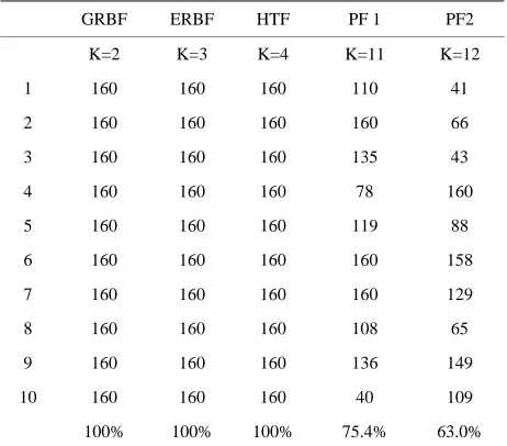
100% 100% 100% 75.4% 63.0%
Table 6. Classification results for oscillation transient.
GRBF ERBF HTF PF 1 PF2
K=2 K=3 K=4 K=11 K=12
1 160 160 160 136 85
2 160 160 160 148 53
3 160 160 160 97 137
4 160 160 160 95 70
5 160 160 160 75 157
6 160 160 160 119 113
7 160 160 160 80 81
8 160 160 160 140 88
9 160 160 160 129 160
10 160 160 160 87 72
100% 100% 100% 69.1% 63.5%
7 6
[image:4.595.58.286.355.528.2] [image:4.595.60.287.556.736.2] [image:4.595.308.539.560.736.2]u lass cla r with RBF, and HTF itab cla g s s of electric po
sforms to decompose electric power into 11 layers and extract each layer’s
REFERENCES
[1] A. M. Gaouda, M. M M. R. Sultan “Power Qual assification Using
The m lti-c SVM ssifie G ERBF, are su le for ssifyin ix type
wer disturbances. By contrast, PF should not be used to solve such disturbances. As indicated by the results, the choice of kernel function considerably influences the classification results of multi-class SVM.
5. Conclusions
Using wavelet tran disturbance signals
detail coefficients as feature vectors can improve the accuracy of classification results. In classifying different types of electric power disturbance signals, the suitable kernel functions for multi-class SVM algorithms are GRBF, ERBF, and HTF. Multi-class SVM classification combined with wavelet transform can be an efficient method for differentiating power quality disturbance signals.
. A. Salama and ity Detection and Cl
,
Wavelets Multi-resolution Signal Decomposition,” IEEE Trans on Power Delivery, Vol. 14, No. 4, 1999,pp. 1469-1476.doi:10.1109/61.796242
[2] Y. Liao and J. B. Lee, “A Fuzzy-expert System for Clas sifying Power Quality Disturbances,” International Jour-nal of Electrical Power and Energy Systems, Vol. 26, No. 3, 2004, pp.199-205.doi:10.1016/j.ijepes.2003.10.012
[3] J. L. Yi and J. C. Peng, “Classification of Short-time
Power Quality Disturbance Signals Based on Generalized S-transform,” Power System Technology, Vol. 33, No. 5, 2009, pp. 22-27.
[4] Y. F. Ren, H. S. Li and H. T. Hu, “Parallel Power Quality
M. Zhou, “Short-time Power
ng and B. Y. Wen, “Identification of Power
d T. Lobos, “Automated Classification of Pow-Controller Based on Multilayer Feedforward Neural Net-work,” Transactions of China Electrical Society, Vol. 22, No. 8, 2007, pp. 108-113.
[5] G. Y. Li, H. L. Wang and
Quality Disturbances Identification Based on Improved Wavelet Energy Entropy and SVM,” Transactions of China Electrical Society, Vol. 24, No. 4, 2009, pp. 161-167.
[6] G. H. Ya
Quality Disturbance Based on QPSO-ANN,” Journal of China Motor Engineering, Vol. 28, No. 10, 2008, pp. 123-129.
[7] P. Janik an
er-quality Disturbances Using SVM and RBF Networks,” IEEE Transaction on Power Delivery, Vol. 21, No. 3, 2006, pp. 1663-1669.doi:10.1109/TPWRD.2006.874114
[8] J. G. Yao, Z. F. Guo and J. P. Chen, “A New Approach to
sification
ng and L. liu, “Improvement on Bin-Recognize Power Quality Disturbances Based on Wavelet Transform and BP Neural Network,” Power System Technology, Vol. 36, No. 5, 2012, pp. 139-144.
[9] N. Hamzah, F. H. Anuwar and Z. Zakaria, “Clas of Transient in Power System Using Support Vector Ma-chine,” 5th international colloquium on signal processing & its applications, Kuala Lumpur Malaysia:IEEE, 2009, pp. 418-422.
[10] Z. Wang, C. L. Wa