New Behavior Model and Adaptive Predistortion for Power
Amplifiers
Mingming Gao1, 2, Yue Wu1, *, Shaojun Fang2, Jingchang Nan1, and Shuyang Cui1
Abstract—A three-box model, composed of a triangular memory polynomial, a look-up table, and a cross item among memory times, is proposed for power amplifiers. The model acquired good accuracy and linear effect and reduced the calculation coefficient. Moreover, the paper proposes the GRLS IVSSLMS adaptive predistortion algorithm. This algorithm is based on the structure of indirect learning. This work uses 16QAM signal to drive a strongly nonlinear Doherty amplifier. Experimental results show that the proposed method is suitable for the adaptive predistortion of power amplifiers.
1. INTRODUCTION
With the development of modern communication technology, power amplifier (PA) devices produce strong nonlinearity and memory effects. Predistortion method is proposed for PA, and popular predistortion models are mainly polynomial, neural network, and look-up table (LUT) [1–3]. Polynomial predistortion models include Wiener-Hammerstein model, Volterra series model, and simplified memory polynomial models. The predistortion models based on LUT [4] are two-dimensional, multidimensional, and filter LUT models [5, 6]. Ref. [7] proposed a polynomial model, whereas [8] proposed the general polynomial model. However, the above predistortion algorithms face the same problem in which the PA model cannot be accurately estimated. The DPD (Digital Pre-Distortion) technology can compensate the nonlinear distortion of PA and memory effect by adopting the adaptive algorithm for baseband signal processing part, which requires the use of predistortion parameter identification algorithm for real-time update. Refs. [9–11] included different improvements on existing adaptive algorithms but still have the shortcomings of computational complexity, real-time and deficient factors of noise resistance, low convergence, and large mean square error. A good algorithm is necessary to improve the effect of predistortion linearization [12].
The remainder of this paper is organized as follows. In Section 2, from the perspective of simplifying the PA model, we propose a new simplified three-box PLTC (parallel-LUT-triangular memory polynomial (TMP)-CIMT) model for the behavioral model of nonlinear PA with memory effect and introduce an identification process. In Section 3, an adopting adaptive algorithm GRLS IVSSLMS is proposed. The PA behavior model uses PLTC model, and the predistortion algorithm utilizes GRLS IVSSLMS algorithm for this paper to achieve a good balance between modeling accuracy and predistortion algorithm complexity in Section 4. Finally, Section 5 concludes the paper.
Received 28 November 2018, Accepted 8 April 2019, Scheduled 31 May 2019 * Corresponding author: Yue Wu ([email protected]).
2. PROPOSED MODEL
2.1. PA Three-Box Behavior Model
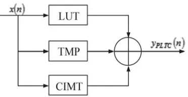
The PLTC model consists of LUT, a TMP, and cross-term memory timing signals in a parallel form. The model obtains a high accuracy by introducing the cross-term of current signals and lagged envelope. The block diagram of the model is illustrated in Figure 1.
Figure 1. The block diagram of the PLTC model.
The first sub-model uses a high-order nonlinear function with memoryless. The PLTC model increases LUT to represent a static strong nonlinearity and reduces the complexity of the entire model. In this work, suppose that x/y is the input and output signals of the first sub-model, Ka a nonlinear order, andak the amplitude. The mathematical expression is written as:
yLUT(n) =
Ka
k=1
akx(n)|x(n)|k−1 (1)
The second sub-model is the TMP function that describes the nonlinear characteristic of an amplifier system. This sub-model is defined by the following formula:
y(n) =
K
k=1 k-odd
Q
qk=0
hk(qk)x(n−q1) (k−1)/2
m=1
x(n−q2m)x∗(n−q2m) (2)
wherekis the number of nonlinear order,qkthe memory depth,hk(qk) thek-order Volterra kernel, and
k= 1,3,· · · , K·qk= 0,1,· · · , Q. The MP is expressed as
y(n) =
K
k=1
Q
q=0
akqx(n−q)|x(n−q)|k−1 (3)
We can attempt to adjust the maximum nonlinear order of the input signal in the past while maintaining the performance of the predistortion and reducing the number of its coefficients. Let
K =N, and N is defined:
N =
K−q; q < K
1; q≥K (4)
From the formula, we can achieve:
yTMP(n) =
Q
q=1
N
k=1
akqx(n−q)|x(n−q)|k−1 (5)
The third sub-model is represented by the memory time signal cross-term CIMT function. The mathematical expression of this sub-model is:
yCIMT(n) =
M
p=1
M
q=1
q=p
N
r=1
cpqrx(n−p)|x(n−q)|r−1 (6)
The increased CIMT model cross-term order will lead to the rapid growth of model coefficients. Considering that the high-order nonlinearity of memory time signals slightly impacts the system, we only consider the impact on the system of three-order intermodulation of the memory timing between signals. Formula (6) is simplified as:
y∗CIMT(n) =
M
p=1
M
q=1
q=p
cpqx(n−p)|x(n−q)|2 (7)
Based on the above analysis, the PLTC model is given as follows:
yPLTC(n) =
Ka
k=1 k-odd
akx(n)|x(n)|k−1+ Q
q=1
N
k=1 k-odd
akqx(n−q)|x(n−q)|k−1
+
M
p=1
M
q=1
q=p
cpqx(n−p)|x(n−q)|2 (8)
The LUT represents the high-order static nonlinear behavior of the PA. The TMP sub-model uses low-order nonlinearity and controls the size of each model separately to form a reasonable number of total coefficients. This model avoids defects in selecting the same nonlinear order in each sub-model, which will increase calculation complexity and size of the model. Therefore, the PLTC model can reduce the size of the model by adding parallel nonlinear sub-models.
2.2. Identification PLTC Model
The PLTC model identification is divided into three steps. First, the high-order memoryless nonlinear static sub-model parameter is identified by the input and output data of the PA. Second, the TMP sub-model parameters are identified. Third, the CIMT sub-model parameters are identified. The TMP sub-model synchronization with the CIMT sub-model is identified as follows:
Y =X·A (9)
where Y is the output vector of two dynamic nonlinear polynomial sub-models,X the matrix of two polynomial basis functions of the input signal, and A the vector that contains the coefficients of the TMP and CIMT sub-model. Matrix X is defined as: X = [XTMP, XCIMT]. The matrix size XTMP is K×((MTMP+ 1)×NTMP) and:
XTMP= [XTMP1,l(x(n0+ 1))· · · XTMPk,l(x(n0+k))]T (10) kis the length of the vector and k= 1000. XTMP,l is defined as:
XTMPk,i+(j×NTMP)(x(n0+k)) =x((n0+k)−j)× |x((n0+k)−j)|
i−1
(11)
j is scanned from 0 to MTMP, and iis scanned from 0 toNTMP. Similarly,XCIMT is defined as: XCIMTk,i+(j×NCIMT)(x(n0+k)) =x(n0+k)× |x((n0+k)−j)|
i−1
(12) Finally, the least squares fitting method is used to calculateA. [ ]H is the conjugate transposition.
The accuracy of each model is measured with normalized mean square error (NMSE). A low NMSE is obtained by selecting low coefficient model dimensions. The sub-model is determined by the size of the general scanning method.
NMSEdB = 10 log10
K
n=1
|ymeans(n)−yest(n)|2
K
n=1
|ymeans(n)|2 (14)
3. PROPOSED ALGORITHM
The DPD technology can compensate the nonlinear distortion of PA and memory effect by adopting adaptive algorithms [13–15], which use predistortion parameter identification algorithms for real-time update. This paper introduces an improved adaptive algorithm for DPD, which adopts the structure of indirect learning.
3.1. I VSSLMS Algorithm
The VSSLMS (variable step size least mean square) algorithm is a class of LMS algorithms with variable step sizes, which overcomes the contradiction between convergence speed and the steady-state error of fixed step size LMS. In this paper, we propose a new VSS LMS, in which X(n) and d(n) stand for the input and output signals;W(n) represents the tap coefficient of the filter; and e(n) is the error signal. The VSS LMS algorithm is expressed as follows.
e(n) = d(n)−XT(n)W(n) (15)
W (n+ 1) = W(n) +μ(n)e(n)X(n) (16) where μ(n) is the variable step size, and the relationship of the updating steps is expressed by Formula (17).
μ(n+ 1) =
⎧ ⎨ ⎩
μmin μ(n)< μmin αμ(n) +βe2(n) other
μmax μ(n)> μmax
(17)
In Formula (17), α determines the convergence step, and it is approximately 1; β determines the degree of influence in error transient energy of the steps and controls the steady-state error and convergence time, and 0 < β < 1. μmax is the maximum possible convergence rate step size, and
the approximate value of μmax is minimal, approximately λmax1 . λmax is the largest eigenvalue of the
correlation matrix of the input signal. μmin is the minimum step, which has the ability to track. e(n) is
approximately zero, and βe2(n) is also close to zero. Hence, the VSS LMS algorithm ensures that the
steady-state error is minimal and that it has a rapid convergence rate and time-varying tracking ability, but is susceptible to noise interference.
The VFSS LMS algorithm is an improved VSS LMS algorithm. p(n) is the estimation error ofe(n) ande(n−1). When the iteration step changes with the average time domain autocorrelation estimate of
e(n) ande(n−1), this step is unaffected by uncorrelated noise impact. The VFSS LMS step algorithm for updating is as follows:
μ(n+ 1) =
⎧ ⎨ ⎩
μmin μ(n)< μmin αμ(n) +βp2(n) other
μmax μ(n)> μmax
(18)
p(n) = γp(n−1) + (1−γ)e(n)e(n−1) (19) where 0 < γ < 1 controls the convergence time, μ(0) = μmax, and p(0) = μ(0). We can ensure that
a faster convergence rate is observed in the initial stage of the adaptive. β is used for controlling the steady-state error of the algorithm and convergence time. However, the noise affects β and makes the step length relatively large. Adding to the time-varying β, which changes with the error signal, this paper proposes the idea of an improved I VSSLMS algorithm. The expression is as follows.
μ(n+ 1) =
⎧ ⎨ ⎩
μmin μ(n)< μmin
αμ(n) +β(n)e2(n) other
μmax μ(n)> μmax
(21)
First,β is large and can obtain a high step value influenced by the error signal. When the algorithm gradually turns into a steady state, β decreases with the declining error signal, and β obtains a low step value to ensure a steady state. When the system impulse response changes, the error signal rapidly changes, and the influence ofβ enlarges, which makes the step length change quickly in order to sustain the change of the system with the change of the system. We illustrate the algorithm performance by experiment.
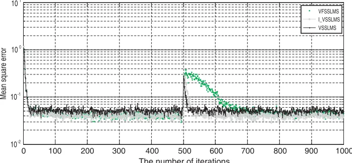
The steps of the performance verification of the adaptive filter algorithm are as follows: (1) adaptive filter order L = 2; (2) signal X(n) is a white Gaussian noise of zero mean with a variance of 1; (3)
v(n) andX(n) are associated with the white noise sequence with zero mean, and variance is 0.04; (4) algorithm sampling for 1000 times; the coefficient of the unknown system changes w1 = [0.8,0.5]T
into w2 = [0.4,0.2]T for 500 times; the VSS LMS algorithm parameters take α = 0.98, β = 0.08, γ =
0.98, μmax = 0.2, μmin = 0. To obtain a learning curve, 200 independent simulations are required with
sampling for 2000 times, and then the mean square error is calculated.
In Figure 2, the VSS LMS algorithm convergence speed is fast, but the steady-state error is also large. The VFSS LMS algorithm steady-state error is minimal but is slow in time-varying tracking. The I VSSLMS algorithm convergence speed is fast, and its steady-state error is minimal.
10-2
10-1
100 101
0 100 200 300 400 500 600 700 800 900 1000
The number of iterations
Mean square error
VFSSLMS I_VSSLMS VSSLMS
Figure 2. VSS LMS algorithms learning curve comparison chart.
3.2. Improved RLS Algorithm
The RLS algorithm has the advantages of rapid convergence and minimal steady-state offset error, but its computing cost is relatively large and unstable when the error signal is less. Thus, improving the traditional RLS algorithm is necessary. The cost function of RLS is as follows.
F(e(n)) =
n
i=0
λn−ie2(n) =
n
i=0
λn−id(n)−XT(n)W(n)2 (22)
where λis known as the forgetting factor, and 0< λ <1. The RLS algorithm weight vector iteration formula is:
W(n) = W(n−1) +K(n)e(n) (23)
K(n) = R
−1(n−1)X(n)
where K(n) is the Kalman gain vector. The B RLS algorithm is based on basic variable forgetting factor, which solves the contradiction between convergence speed and steady-state error. The B RLS algorithm is expressed as:
λ(n) = λmin+ (1−λmin)·2L(n) (25)
L(n) = −round[ρe2(n)] (26) where round(·) is the nearest integer, and ρ controls the sensitivity of the estimation error. First,e(n) is large, andλ(n) is λmin to ensure rapid tracking. When the system is stabilized,e(n) is smaller, and λ(n) is 1 to ensure a minimal steady-state error. When the system is unknown,K(n) trends become 0, and then the system is not updated.
A self-perturbation term becomes the Z RLS algorithm through the inverse covariance matrixP(n), avoiding K(n) becoming 0. The formula to updata P(n) is as follows.
P(n) = 1
λ
P(n−1)−K(n)XT(n)P(n−1) + round[γe(n)] (27) where γ is the sensitive factor by taking γ = 1, and round [γe(n)] is the nearest integer to γe(n). Adopting e(n) as a self-disturbance, this phenomenon makes the algorithm concise. Given that the expectations e(n) and noise signal unrelated, this condition enhances the anti-noise interference ability of the Z RLS algorithm. This paper proposes an improved RLS algorithm (G RLS), which combines genetic factor and disturbance.
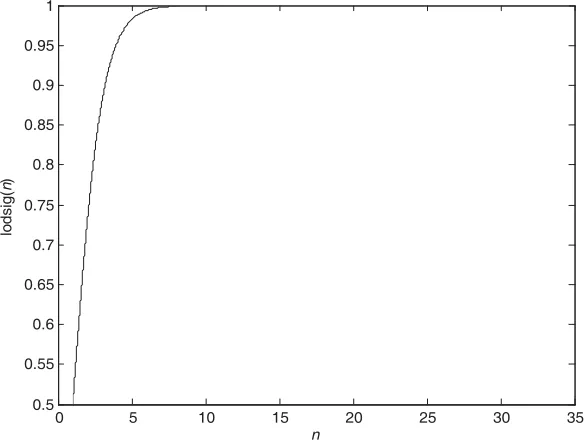
The G RLS algorithm adjustsλthrough function log sig(·). λincreases with the number of trainings while strengthening the tracking ability and reducing the estimation error. In this work, the change of
λrelated to the number of iterations ignores the error signal, and the algorithm is slightly susceptible to the effects of interference noise. The forgetting factor is expressed as Formula (28).
λ(n) =λmin+ (1−λmin)×log sig(n/M) (28)
wherenis the number of iterations;M is an integer;λmin,n, andM can be obtained by the experiment.
The function y= log sig(x) is expressed by Formula (29) and illustrated by Figure 6.
y= 1/1 +e−x (29)
In Figure 3, the iteration is few, andλis minimal, making the convergence of the algorithm fast. When the algorithm converges into a steady state with the increase of the number of iterations, λ is large, and the steady-state error is minimal.
0 5 10 15 20 25 30 35
0.5 0.55 0.6 0.65 0.7 0.75 0.8 0.85 0.9 0.95 1
n
lo
dsig
(
n
)
The improved G RLS algorithm is combined with the Z RLS algorithm, and the improved forgetting factor method can obtain good convergence speed and steady-state error performances. The G RLS algorithm is expressed as follows.
λ(n) = λmin+ (1−λmin)×log sig(n/M) (30) P(n) = 1
λ(n)
P(n−1)−K(n)XT(n)P(n−1) + round[γe(n)] (31)
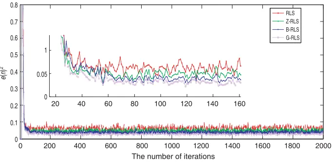
The learning curve comparison chart of the RLS algorithm is illustrated in Figure 4. The parameter settings are described above, and the G RLS algorithm λmin = 0.95, M = 60. The figure shows that
the G RLS algorithm is the best, since its convergence speed is the fastest, and the steady-state error is the smallest.
0 200 400 600 800 1000
The number of iterations
1200 1400 1600 1800 2000
0.8
0.7
0.6
0.5
0.4
0.3
0.2
0.1
0
e
(
n
)
2
20 40 60 80 100 120 140 160
1
0.05
0
RLS Z-RLS B-RLS G-RLS
Figure 4. RLS algorithms learning curve comparison chart.
3.3. GRLS IVSSLMS Algorithm
The RLS LMS takes the advantages of both LMS and RLS algorithms; therefore, it has a rapid convergence rate and minimal steady-state error. This paper proposes the GRLS IVSSLMS algorithm, which further improves the performance of the RLS LMS algorithm and PD effect. The GRLS IVSSLMS algorithm learning curve comparison chart is depicted in Figure 5. The RLS algorithmμ= 0.01,ET = 0.5, and the LMS algorithm μmax = 0.65. In the remaining parameters described above, the
GRLS IVSSLMS algorithm has a good convergence speed and steady-state misadjustment.
4. RESULT AND DISCUSSION
The design of the proposed adaptive algorithm is based on the initial stage of convergence or an unknown system parameter change. The step size should be relatively large to obtain rapid convergence speed and tracking speed time-varying systems. The algorithm converges should be kept minimal to achieve the small step size of the steady-state offset noise regardless of the primary input interfering signalv(n). The adaptive predistortion system block diagram of the GRLS IVSSLMS algorithm is illustrated by Figure 6. The PA using the PLTC model and the PD algorithm using the GRLS IVSSLMS select the G RLS algorithm in the initial phase. After the steady-state of the G RLS algorithm, the switch automatically receives the second side and converts to the I VSSLMS algorithm. When the error is more than the threshold, the algorithm switches to receive the first side, and then repeats the above process. The error signal threshold is important. Let ET = |e(n)|, the threshold ET is unaffected by other factors. The algorithm is only related to the error signal and can ensure stability.
10-1
100
0 200 400 600 800 1000
The number of iterations
1200 1400 1600 1800 2000
e
(
n
)
2
RLS_LMS GRLS_IVSSLMS
Figure 5. GRLS IVSSLMS algorithm learning curve comparison chart.
~
x(n) z(n) y(n)
e(n)
z(n)
Figure 6. DPD system block diagram of the GRLS IVSSLMS algorithm.
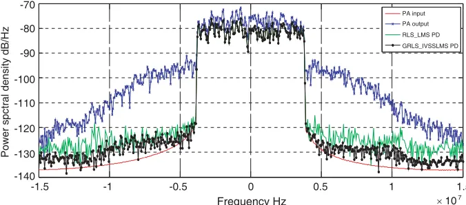
-1.5 -1 -0.5 0 0.5 1 1.5
Frequency Hz × 107
-70
-80
-90
-100
-110
-120
-130
-140
Power spctral density dB/Hz
PA input PA output RLS_LMS PD GRLS_IVSSLMS PD
Figure 7. Spectrum comparison chart after the GRLS IVSSLMS PD algorithms.
GRLS IVSSLMS PD algorithm is improved by approximately 29 dB compared with the predistortion PA output.
-8 -6 -4 -2 0 2 4 6 8
(a) (b)
0 0.1 0.2 0.3 0.4 0.5 0.6 0.7
Input amplitude
0 0.1 0.2 0.3 0.4 0.5 0.6 0.7
Input amplitude 0
0.1 0.2 0.3 0.4 0.5 0.6 0.7
Output amplitude Output phase
PA LMS RLS GRLS_IVSSLMS
PA LMS RLS GRLS_IVSSLMS
Figure 8. AM/AM and AM/PM characters after the GRLS IVSSLMS PD algorithm. (a) AM/AM. (b) AM/PM.
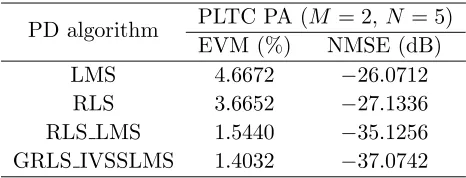
Table 1. GRLS IVSSLMS algorithm performance comparison.
PD algorithm PLTC PA (M = 2,N = 5) EVM (%) NMSE (dB) LMS 4.6672 −26.0712
RLS 3.6652 −27.1336 RLS LMS 1.5440 −35.1256 GRLS IVSSLMS 1.4032 −37.0742
effect is greatly improved and can meet the system requirements.
In Table 1, compared with the LMS, RLS, and RLS LMS algorithms, the EVM of the proposed method is improved by 3.26%, 2.26%, and 0.14%, respectively, whereas the NMSE of the proposed method is improved by 11, 9.9, and 1.95 dB, respectively.
5. CONCLUSION
The increasing demand of testing large-scale real-world programs necessitates the automation of the testing process. As a basic problem in software testing, path-wise test data generation is particularly important. We proposed a look-ahead search method in our previous research, and in this paper we make improvements on interval arithmetic, which enforces arc consistency. We analyze, in detail, the working process of interval arithmetic, and based on the analytical result, the iterative operator is introduced and adopted in the constraint solving process, for the purpose of detecting infeasible paths as well as shortening the time consumption. Experimental results prove the effectiveness of the iterative operator and its applicability in engineering.
Our future research will involve how to make interval arithmetic more efficient in arc consistency checking. We will also introduce more arc consistency checking techniques and more ways of representing the values of variables such as affine arithmetic. The MC/DC coverage criterion will be given more emphasis. We will continue to improve the effectiveness of the generation approach and provide better support for more data types.
ACKNOWLEDGMENT
This work was supported by the National Natural Science Foundation of China Youth Fund Project (No. 61701211), Liaoning Provincial Key Laboratory Funding Project (NO. LJZS007), and Liaoning Provincial Department of education general project (L2015209).
REFERENCES
1. Zhang, L., “Three-dimensional power segmented tracking for adaptive digital pre-distortion,”
IEICE Electron. Express, Vol. 13, 1, 2016, doi: 10.1587/elex.13.20160711.
2. Mkadem, F., et al., “Multi band complexity reduced generalized memory polynomial power-amplifier digital predistortion,” IEEE Trans. Microw. Theory Techn., Vol. 64, 1763, 2016, doi: 10.1109/TMTT.2016.2561279.
3. Hammi, O., et al., “Multi-basis weighted memory polynomial for RF power amplifiers behavioral modeling,”IEEE MTT-S International Conf., Vol. 1, 2016, doi: 10.1109/IEEE-IWS.2016.7585475. 4. Ba, S. N., K. Waheed, and G. T. Zhou, “Efficient lookup table-based adaptive baseband predistortion architecture for memoryless nonlinearity,” EURASIP Journal on Advances in Signal Processing, 379249, 2010, doi: 10.1155/2010/379249.
5. Chen, H. H., et al., “Joint polynomial and look-up-table predistortion power amplifier linearization,”IEEE Trans. Circuit System, Vol. 53, 612, 2006, doi: 10.1109/TCSII.2006.877278. 6. Yang, Z., et al., “PA linearization using multi-stage look-up-table predistorter with optimal
linear weighted delay,” IEEE International Conf. Signal Process., Vol. 47, 2012, doi: 10.1109/ICoSP.2012.6491529.
7. Kim, J., et al., “Digital predistortion of wideband signals based on power amplifier model with memory,”Electronics Letters, Vol. 37, 1417, 2001, doi: 10.1049/el:20010940.
8. Morgan, D. R., et al., “A generalized memory polynomial model for digital predistortion of RF power amplifiers,” IEEE Transactions on Signal Processing, Vol. 54, 3852, 2006, doi: 10.1109/TSP.2006.879264.
9. Yao, S., et al., “A recursive least squares algorithm with reduced complexity for digital predistortion linearization,” IEEE International Conf. Signal Process., 4736, 2013, doi: 10.1109/ICASSP.2013.6638559.
10. Mandic, D. P., “A generalized normalized gradient descent algorithm,” IEEE Signal Processing Letters, Vol. 11, 115, 2004, doi: 10.1109/LSP.2003.821649.
11. Liu, Y. J., et al., “A robust augmented complexity-reduced generalized memory polynomial for wideband RF power amplifiers,” IEEE Trans. on Industrial Electronics, Vol. 61, 2389, 2014, doi: 10.1109/TIE.2013.2270217.
12. Dawar, N., T. Sharma, R. Darraji, and F. M. Ghannouchi, “Linearisation of radio frequency power amplifiers exhibiting memory effects using direct learning-based adaptive digital predistoriton,”
IET Communications, Vol. 10, No. 8, 950–954, May 19, 2016, doi: 10.1049/iet-com.2015.1048. 13. Carusone, A. C., “An equalizer adaptation algorithm to reduce jitter in binary receivers,” IEEE
Transactions on Circuits and Systems II: Express Briefs, Vol. 53, No. 9, 807–811, Sep. 2006, doi: 10.1109/TCSII.2006.881161.
14. Akhtar, M. T., M. Abe, and M. Kawamata, “A new variable step size LMS algorithm-based method for improved online secondary path modeling in active noise control systems,” IEEE Transactions on Audio, Speech, and Language Processing, Vol. 14, No. 2, 720–726, Mar. 2006, doi: 10.1109/TSA.2005.855829.