ENSEMBLE SELECTION AND OPTIMIZATION BASED ON SOFT SET THEORY FOR CUSTOMER CHURN CLASSIFICATION

(1)

ISSN: 1992-8645 www.jatit.org E-ISSN: 1817-3195

45

PARAMETER ESTIMATION OF GEOGRAPHICALLY

WEIGHTED MULTIVARIATE t REGRESSION MODEL

1

HARMI SUGIARTI, 2PURHADI, 3SUTIKNO, 4SANTI WULAN PURNAMI

1

Department of Statistics, Universitas Terbuka, Tangerang Selatan, Indonesia

234

Department of Statistics, Institut Teknologi Sepuluh Nopember, Surabaya, Indonesia E-mail: [email protected], [email protected], [email protected],

4

[email protected]

ABSTRACT

The use of ordinary linear regression model in spatial heterogeneity data often does not suitable within the data points, especially the relationship between response variable and explanatory variables. Therefore, the geographically weighted t regression (GWtR) is used to overcome spatial heterogeneity term. The model is an extension of geographically weighted regression (GWR) which the response variable follows multivariate t distribution. The aim of this study is to obtain the estimator of geographically weighted multivariate t regression (GWMtR) model with known degrees of freedom. The maximum likelihood estimation (MLE) method will be applied to maximize a weighted logarithm likelihood function. Based on the EM algorithm, the estimator of geographically weighted multivariate t regression model can be determined.

Keywords: Maximum Likelihood Estimation (MLE), EM Algorithm, Geographically Weigted Regression, Multivariate t Model

1. INTRODUCTION

The linear regression model are often used to describe the relationship between the response variable and the independent variable. The estimation of linear regression model by the ordinary least squares (OLS) method can be used when the error has normal distribution. A number of studies of multivariate t linear regression were performed. A study of univariate linear regression and multivariate linear regression are developed to obtain a robust linear regression model when data follow the heavy tail distribution. The maximum likelihood estimation (MLE) method can be applied to find the mean and covariance matrix of estimator robust. In addition, it is suggested to treat the degrees of freedom of t distribution as a known parameter when the sample size is small and to estimate it when the sample size is large [1].

Although, MLE method and Bayesian method have a weakness when the data have null probability under sampling model assumption, the inference of multivariate t linear regression with unknown degrees of freedom was developed. Fernandez and Steel [2] suggested that Bayesian

analysis is based on a set of observations with the accuracy of the initial data. MLE method is not recommended without further study of the properties of the local maxima when it is used to find the estimator of model with errors multivariate t distribution and unknown degrees of freedom.

Liu and Rubin [3] developed a maximum likelihood method using EM algorithm to estimate the parameters of the multivariate t regression model with known and unknown degrees of freedom. The algorithm has analytically quite simple and has stable monotone convergence to a local maximum likelihood estimate.

(2)

46 Some studies on models of classical GWR model has been discussed, where an error follows a normal distribution. Although Lu, et al. [5] proposed non-Euclidean distance (non-ED) metrics calibrated with Euclidean distance (ED), road network distance and travel time metrics in GWR model, but the error still follows a normal distribution.

An early review of the GWtR model has been done by Sugiarti, et al. [6]. The study indicates that the parameters of the model GWtR can be estimated by maximum likelihood method. The method maximize the weighted logarithm likelihood function of the response variable and get the value of the estimator using the Newton-Raphson iteration. In this paper we propose the maximum likelihood estimator of geographically weighted multivariate t regression model with known degrees of freedom using EM algorithm.

2. MULTIVARIATE t DISTRIBUTION

Base on Nadarajah and Dey [7], vector yi is said

to have the q-variate t distribution with degrees of freedom

ν

, mean vector µ , and scale matrix Ψ, if its probability density function (pdf) is given by:

( )

2 1

2 2

( ) 1

( )

q

i i

D f

ν

πν

+

− +

Γ  

= _ + _

Γ  

y

θ

Ψ (1)

where

( )

₍ ₎T 1₍ ₎

i i i

D θ = y −µ Ψ− y −µ ,−∞< <∞y_i ,

−∞< <∞µ , Ψ>0, and ν>0.

An illustration of bivariate t distribution with

ν

=2,

0 =

µ , and 1 0.4 0.4 1

 

 

 

Ψ = is shown in Figure 1.

Figure 1: Bivariate t Distribution with v=2

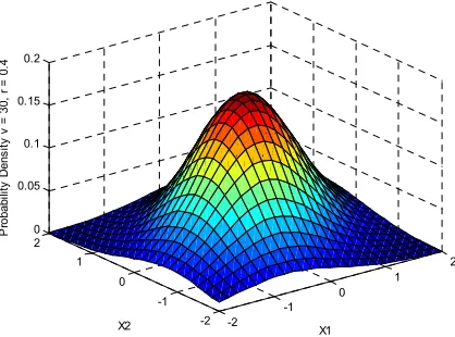
[image:2.612.321.530.162.317.2]

The bivariate t distribution has havier tail than Normal distribution. It can be shown when degrees of freedom

ν

=30 is increased as in Figure 2.

Figure 2: Bivariate t Distribution with v=30

The expectation and variance of vector yi can be

expressed by:

( )

; var

( )

; 2

2

i i

E

ν

 

= =_ _ >

−

 

y

µ

y Ψ

3. MULTIVARIATE t REGRESSION

Multivariate t regression model is developed based on multivariate regression model with response variables that follow multivariate t distribution. Suppose q response variables

1 2

( ,Y Y,K,Y_q)_{associated with} _p_independent variables (X X₁, ₂, ,KX_p)_{can be written as:}

( 1)

( 1) ( 1) 1 ( 1)

; 1,2,...,

T

i _q _p i i

q p q

i n

× +

× + × ×

= + =

y Β x ε

(2)

1 01 11 1

2 02 12 2

( 1) ( 1)

0 1

; ;

i p

i T p

i

q p q

q q pq

iq Y Y

Y

β β β

× +

×

   

   

=_ _ =_ _

  _ _

  _ _

 

L L

M M O M

M

L

y Β

1

1 2

( 1) 1 ( 1) 1

;

i

i i

p q

ip iq

X

ε ε

ε

+ × ×

 

 

=_ _ _{=  }

 

   

   

M M

x ε

Vector yi follows theq-variate t distribution with

degrees of freedom

ν

, mean vector T i x

Β and scale

-2 -1

0 1

2

-2 -1 0 1 2 0 0.05 0.1 0.15 0.2

X1 X2

P

ro

b

a

b

ili

ty

D

e

n

s

it

y

v

=

3

0

,

r

=

0

(3)

47 matrix Ψ. The probability density function (pdf) of vector y_i is given by:

( )

2 1

2 2

( ) 1

( ) q q q i i D f ν ν ν

ν

πν

+ − +

Γ _ _

= _ + _

Γ  

y

θ

Ψ (3)

where

( )

₍ T ₎T 1₍ T ₎

i i i i i

D θ = y −Β x Ψ− y −Β x is Mahala-nobis distance. The expectation and variance of vector yi can be denoted by:

( )

; var

( )

; 2

2

T

i i i

E

ν

 

= =_ _ >

−

 

y

Β

x y Ψ

Based on equation (3), the likelihood function can be stated as

( )

2 2 2 1 2 1 2 ( ) ( ) 1 ( ) q qn n n i i n q n i n i f D ν ν ν

ν

πν

+ = + − = =

Γ  _ _

 

= _ + _

Γ   

 

∏

l

θ

_y

θ

Ψ

(4)

The maximum likelihood estimation of parameter multivariate t regression can be obtained by the maximized of logarithm likelihood function

( )

2 2 2 1

ln ( ) ln ln

2 ( ) ln 1 2 q q n i i n n D q ν ν

πν

ν

+ = Γ = − Γ   +   − _ + _    

∑

l

θ

Ψ (5)

Furthermore, assuming that the likelihood function is differentiable, the estimator can be found by solving the simultaneous equations below.

ln ( )

∂

=

∂ 0

lθ

Β and

ln ( )

∂

=

∂ 0

lθ

Ψ (6)

Differentiating with respect to

Β

and Ψ, respectively is given by

[

]

(

)

[

]

1 1 1 1 1 1 ( )

ln ( )

( ) ( ) ( ) ( ) T T n

i i i

i i

T T n

i i i

i i

n

T T i i i i i q D q D ν ν ν ν ω − = − = − = − ∂ _{= +} ∂ + + − = + = −

∑

lθ Β

Β θ Β θ Β Ψ Ψ Ψ

x y x

( )

1 1 1 1 1 1 1 1 1 1 ln ( ) 1

2 2 1 1 2 1 2 n i ij T i i ij n i i n i ij n T

i i i

ij i tr q D tr σ σ ν _ν ν σ ω σ − = − − = − = − − = ∂ _{= −}  ∂    ∂ _ ∂ _ ∂ ₋   _∂    + − + ∂   = − _ _ ∂   ∂   + _ _ ∂  

∑

lθ ε ε θ ε ε Ψ Ψ Ψ Ψ Ψ Ψ Ψ Ψ Ψ Ψ Ψ where

( )

i i q D ν ω ν + =

+ θ ,

T i i− i

ε = y Β x , and

ij

σ

∂ ∂

Ψ

is the symmetric q q× matrix that has ones in row i column j and row j column i, and zeros elsewhere.

Since the equation (6) does not result in closed form solution, the estimator of

Β

and Ψ can be determined by the iteratively process. Liu and Rubin [3] used the EM algorithm to obtain the maximum likelihood estimator that consists of E-step (Estimation E-step) followed by M-E-step (Maximization step). The E-step of the EM algorithm aims to obtain the conditional expectation of the complete data sufficient statistics when given the observed values. The M-step involves weighted least squares estimation of

Β

and Ψ. Thus, the EM algorithm iterates successively until the convergence is reached.

At iteration (r+1) with input _Β( )r

and _Ψ( )r

, the E-step of EM algorithm calculate the expectation of ln likelihood complete and the expected sufficient statistics, respectively as follows:

( 1) ( ) ( ) r i r i q D

ν

ω

ν

+ ₌ +

+

θ

and

( ) _ˆ( ) ˆr ₌ r

y X B

( )

( 1) ( 1)

1

( 1) ( 1) ( ) 1

( 1) ( 1) ( ) ( ) ( )

1 1

ˆ

1 ˆ ˆ

n

r r T

XX i i i i

n

T

r r r

XY i i i i

n n

T

r r r r r

YY i i i i

i i S S S n ω ω ω ω ω ω + + = + + = + + = = = = = +

∑

Ψ

x x x y

y y

(7)

The M-step of EM algorithm will calculate

(

)

(

) (

)

1 ( 1) ( 1) ( 1)

1 ( 1) ( 1) ( 1) ( 1) ( 1)

ˆ

1 ˆ

r r r

XX XY T

r r r r r

i YY XY XX XY

S S

S S S S

n

ω ω

ω ω ω ω

(4)

48 4. GEOGRAPHICALLY WEIGHTED

MULTIVARIATE t REGRESSION

Geographically weighted multivariate t regression (GWMtR) model is developed based on geographically weighted t regression (GWtR) model which proposed by Sugiarti et al. [6]. The model describes relationship between q response variables y_i and p independent variables x_i by considering the location factor that expressed as vector coordinate in two dimensional of geographic space. Hence, the estimator obtained in GWMtR model is a local estimator for each point of observation. Let ui =(u ui1, i2) is a coordinate in two dimensional geographic space (latitude and longitude), the expectation of GWMtR model can be defined as follows:

( )

( 1) 1 ( 1) ( 1)

; 1, 2,...,

T

i i i

p q q p

E i n

+ ×

× × +

= =

y Β u x (9) where

1

1 2

( 1) ( 1) 1

1

; ;

i

i i

q p

ip iq

Y

X Y

× + ×

   

   

=_{ } =_ _

 

  _ _

 

M M

y x

( )

01 11 1

02 12 2

( 1)

0 1

i i p i

T i q p

q i q i pq i

β β β

× +

 

 

=_ _

 

 

L L

M M O M

L

Β

u u u

u

u u u

and vector

(

T

( )

,

( )

,

)

itq i i i ν

y Β u x Ψu have the q -variate t distribution and probability density function is

( )

(

)

2

1

2 2

( ) 1

( )

q

i i i

i

D f

ν ν

πν

+ − +

Γ  

= _+ _

 

Γ

u y

u

θ

Ψ

(10)

where

( )

(

)

(

_T

( )

)

T

(

( )

)

1

(

_T

( )

)

i i i i i i i i i

D

θ

u = y−

Β

u x Ψu − y−

Β

u x

5. PARAMETER ESTIMATION OF GEOGRAPHICALLY WEIGHTED MULTIVARIATE t REGRESSION

Maximum likelihood estimation of parameter GWMtR model can be obtained by the maximized of weighted logarithm likelihood function (10).

( )

(

)

( )

(

)

1

2 2

* *

1

2 *

1

2

* *

1

ln ( )ln ( )

( ) ln ( ) ( ) ln 1

2

q

n

i i i i

i

q n

i i i

n

i i i i

i

w f

w

D q

w

ν ν

πν ν

ν ∗

=

+

=

 _Γ 

 

=  

 Γ 

 

 

+

 

− _ _{ }+ 



∑

l θ

θ

u u y

u

u u

Ψ

(11) where w_i

( )

u_i_* is a weighted function for locationui

and

(

( )

)

( )

1

( )

* ( * ) * ( * )

T T T

i i i i i i i i i

Dθ u = y−Β u x Ψ− u y−Β u x

There are some types of weighting functions that can be used to describe the relationship between the observations at the location i to other locations. The one obvious choice is the Gaussian function [8]

( )

* 2

*

1 exp

2

ii i i

d w

h

 _ _ 

= _− _ _ _

 

u (12)

(

) (

2

)

2

* * *

ii i i i i d = u −u + v−v

where d_ii_* is Euclidean distance between location *

i and location i with bandwidth h.

Lu, et al. [5] propose non-Euclidean distance (non-ED) metrics calibrated with Euclidean distance (ED), road network distance and travel time metrics in GWR model. The results indicate that GWR calibrated with a non-Euclidean metric can not only improve model fit, but also provide additional and useful insights about relationships within data set. However, Lu, et al. [9] propose a back-fitting approach to calibrate a GWR model with parameter-specific distance metrics. The results show that the approach can provide both more accurate predictions and parameter estimates, than that found with standard GWR.

In order to select an appropriate bandwidth in GWR, there are a number of criteria that can be used, one of them is generalized cross validation criterion (GCV) which is described Matsui, et al.

[10]

( )

[

]

[

( )

]

{

}

( )

(

)

( )

2 1 1 1

ˆ ˆ

1

T

T T

i i

trace h h

GCV

n q v

n q

v trace −

− −

=

 ₋ 

 

 

=

y y y y

X W u X X W u

(5)

49 where yˆ( )h is the fitted value of y( )h using a bandwidth of h, W u

( )

_i is weighted matrix that consists weighting function in equation (12).

Estimation of GWMtR's parameter model is obtained through the following equation.

( )

(

)

( )

* *

ln i

i

∗ ∂

=

∂ 0

l θ

Β

u

u and

( )

(

)

( )

* *

ln i

i

∗ ∂

=

∂ 0

l θ _u

u

Ψ (14)

Differentiating with respect to Β

( )

u_i_* and Ψ

( )

u_i_* , respectively is given by

( )

(

)

( )

(

)

( )

(

)

1

* *

1

* *

ln _n T

i i i i i

i

i i i

q w D ν

ν

∗ −

= =

∂ +

∂

∑

+

l θ _ε

Β θ

u u x

u u

Ψ

( )

(

)

( )

( ) ( )

( )

1

* *

1 *

* * *

1

ln 1

2

1 2

n

i i

i i i

i

i ij

n

T

i i i i i i i i

w tr

w

σ

ω ∗

−

=

∂  ∂ 

= − __ __

∂ _ ∂ _

 

−_{ } Φ

 

∑

l θ

ε ε

u u

u

u u u

Ψ Ψ

Ψ

(15) where

( )

(

₍

_{( )}

)

₎

( )

* *

*

1 * 1

* * *

T

i i i i

i i

i i i

ij

q

D

ν

ω

ν

σ

− −

= −

+ =

+ ∂

Φ =

∂

ε

Β

θ

y u x

u

u Ψ u Ψ Ψ u

Since the equation (14) does not result in closed form solution, the estimator of Β

( )

u_i_* and Ψ

( )

u_i_*

are determined by the iteratively process.

A joint iterative process to solve (14) is given by EM algorithm. The EM algorithm is developed to maximize the weighted ln likelihood observed through the weighted ln likelihood complete. Let

iτi

y has multivariate normal distribution and τ_i has Gamma distribution with density function, respectively as follows:

(

)

( )

1 2 2

1

1 2

2 1

2 exp ;

2 exp

2 2 2

q

T

i i i i

i i

i

i i

f e e

f

ν ν

τ π

τ τ

ντ

ν ν

τ τ

− −

−

 _{ } 

 

= _− _{ } _

 

 

 

      

= Γ_ _{   }_ _− _

     

 

y Ψ u Ψ u

where e

( )

u_i =

(

y_i−ΒT

( )

u x_i _i

)

Joint density function between y_iτ_i and τ_i can be expressed by

(

) ( )

( )

(

)

1

2 2

1

1 2

2

, 2

2 2

exp 2

q q

i i i

i

i i

f

D

ν _ν

ν ν

τ π τ

τ ν

− + ₋

     

=_ _{Γ } _ _{ }

   

 

₋ _ ₊ _

  

 

y

u

θ Ψ

(16)

Therefore, the τ_i y_i follows Gamma distribution with parameter: ,

(

( )

)

2 2

i i

D qν

ν +

 + 

 

 

u

θ

with its density function can be expressed by

(

)

(

( )

)

( )

(

)

1 2

2

exp 2

2 2

q

i

i i i

i i q

i i

D f

D q

ν

τ

τ ν

τ

ν ν +

−

+ −

₋ _ ₊ _

  

 

=

+

 

+

 

Γ_ __ _

 _ _

u y

u

θ

(17)

The expectation of τ_i y_i can be denoted as:

(

i i

)

₍

_{( )}

₎

i i

q E

D

ν

τ

ν

+ =

+

y

u

θ

(18)

From (16), the weighted ln likelihood complete is given by

( )

(

)

( )

(

)

( ) ( )

( )

(

( )

)

( )

1

2 2

* *

1 * 1

* *

1

1 2

2 *

1

ln ln ,

ln 2 1

2

ln

2 2

q

n

c i i i i i

i n

i i i

n

i i i i i i

n _q

i i _i

i

w f

w

w D

w

ν ν

τ

π

τ ν

ν ν

τ ∗

=

− ₊

−

=

 

=− _ _

− _ + _

_ _{   }_ 

+ _Γ_{   }_ 

     

 

∑

l u u y

u

u u

u

θ

Ψ

(19)

Based on the conditional expectation of τ_i y_i , the E-step of EM algorithm will calculate the expectation of weighted ln likelihood complete. Becauseτ_iunknown, the use of E

(

τ_i y_i

)

is easier than the of E

( )

τ_i .

Hence, at iteration (r+1) with input

( )

(

( )

)

( ) ( ) ( ) ,

r r r

i i i

(6)

ISSN: 1992-8645 www.jatit.org E-ISSN: 1817-3195 50

( )

(

( )

)

( )

(

)

( )

(

( )

)

( )

( 1) ( )

* *

( ) *

( 1) ( )

* * 1 ( 1) * * 1 ( ) * * 1 r r

i i i i

r i i n

r T r

YY i i i i i i i i

n

r T

i i i i i i i

n

r i i i i i

E q D

S w E

w w ω ω τ ν ν τ ω + + = + = = = Θ + = + = Θ = +

∑

θ Ψ u u u

u u y y u

u u y y

u u

( )

(

( )

)

( )

(

( )

)

( )

( 1) ( )

* * *

1

( 1)

* *

1

( 1) ( )

* * * 1 ( 1) * * 1 n

r T r

XY i i i i i i i

i n

r

i i i i i i i

n

r T r

XX i i i i i i i

i n

r T

i i i i i i i

S w E

w

S w E

w ω ω τ ω τ ω + = + = + = + = = Θ = = Θ =

∑

u u x y u

u u x y

u u x x u

u u x x

(20)

The M-step of EM algorithm will calculate

( )

(

( )

)

1

( )

( 1) ( 1) ( 1)

* * *

ˆ r r r

i SωXX i SωXY i

−

+ ₌ + +

u u u

Β

( )

(

( )

)

(

( )

)

1

(

( )

)

( 1) ( 1) ( 1) ( 1) ( 1)

* * * * *

1

ˆ _r _r _r T _r _r

i i SYY i SXY i SXX i SXY i

n ω ω ω ω

−

+ ₌  + ₋ + + + 

 

u u u u u

Ψ

(21)

The estimator of Β

( )

u_i_* and Ψ

( )

u_i_* can be found by update the E-step and M-step iteratively until the convergence of algorithm is reached.

Lange, et al. [1] used the Fisher Information matrix to determine the estimator of the asymptotic variance-covariance matrix ofΒ

( )

u_i_* . The Fisher Information matrix can be expressed as

( )

(

)

( )

2 * * ln i i E ∗ ∂    =  _∂      l u K u ΒΒ

θ

Β

Let

(

)

2 q i q g ν ν + = + z

,

[

( )

]

12

*

i i i

−

=

z Ψ u ε

( )

[

]

1

2 2

* 1

q

T T

i ij i i i

j − =   =_ _= 

∑



z z ε Ψu ε

The equation (15) can be written as

( )

(

)

( )

(

)

( ) ( )

( )

(

)

( )

1

2 1 * * * 1 * * * * 1

ln _n T

i i i i i i

i

i i i

n

T i i q i i i i q w D w g ν ν − ∗ = − = = +   ∂ _ _ ∂ + = _ _

∑

l u u u x

u u

u u z x

Ψ Ψ ε θ Β θ (22)

Hence, the contribution of the current observation in equation (22) to find estimator of Β

( )

u_i_* is

( )

(

)

( )

[

( )

]

1 2 * * * *

ln _i _T

i i q i i i i i w g ∗ − ∂ = ∂ l _u

u u z x

u Ψ

θ

Β

(23)

Based on Lange, et al. [1], when q declared the dimension ofΨ

( )

u_i_* , then the expectation of some function can be expressed

( )

[

]

1

(

[

( )

]

1

)

* *

1

T

i i

i i i

i i E tr q − −   _ _ =         z z

u z u

z Ψ z Ψ

(

)(

)

2 2 2 2 2 i i q E q q ν ν ν ν ν  _ _  ₌    _ _ _{+ +} ₊ +      z z

(

)

(

)(

)

2 2 2 2 2 2 2 i i q q E q q ν ν ν ν ν    ₌   _{+ +} ₊ +     z z

(

)(

)

2 3 2 2 2 i i q q E q q ν ν ν  _ _  ₌    _ _ + + + +      z z

Furthermore, the Fisher Information matrix can be found through

( )

(

)

( )

[

( )

]

( )

(

)

(

[

( )

]

)

( )

(

)

(

[

( )

]

)

( )

( ) ( )

2 1 2

* 2 2

* * * 1 2 2 2 * * 1 2 2 2 * * 2 1 * ln 1 1 2 T

i i i T

i i i q i i i

i i i i

T

i i i q i i i

T

i i i q i i i

T

i i i i

E w E g

w E g tr

q

w E g tr

q q w tr q

ν

∗ − − − − ∂      ₌    _∂              = _ _   = _ _ +  _{ } _ = _ _{ } _ + +  

l u z z

u z x u x

u z z

u z x u x

u z u x x

u x x

Ψ Ψ Ψ Ψ

θ

Β

Hence, the Fisher Information matrix can be expressed as

( )

(

)

( )

(

( )

)

2 * * 2 1 * * 1 ln 2 j i i n T

i i i i i

i E q w tr q ν ν ∗ − = ∂    =   ∂     +  _{ } _ = _ _{ } _ + +  

∑

l u K u

u u x x

ΒΒ

θ Β

Ψ

(24)

(7)

51



(

_{( )}

)

( )

(

1

( )

)

1 *

1 2

* *

1

ˆ cov

2 _ˆ

i

n

T i i j i i i i

q

w tr

q

ν

− −

−

= =

+ +

  _ _ 

=_ ₊ __

∑

_ _ _

u K

u Ψ u x x

ΒΒ

Β

(25)

6. CONCLUCION

GWMtR model is an extension of geographically weighted regression (GWR) which response variables follow multivariate t distribution. In this model, the response variables will be predicted by independent variables for each location. Therefore, there are many estimator of coefficients regression that depend on the location where the data are observed. Parameter estimation of GWMtR model can be done by maximum likelihood estimation (MLE) method with EM algorithm.

REFERENCES:

[1] K. Lange, R. Little and J. Taylor, "Robust Statistical Modeling Using The t Distribution," Journal of the American Statistical Association, vol. 84, pp. 881-896., 1989.

[2] C. Fernandez and M. F. Steel, "Multivariate Student-t Regression Models: Pitfalls and Inference," The Netherlands, 1997.

[3] C. Liu and D. B. Rubin, "ML Estimation of the t Distribution Using EM and its Extensions, ECM and ECME," Statistica Sinica, vol. 5, pp. 19-39, 1995.

[4] L. Anselin, Spatial Econometrics: Methods and Models, Springer, 1988.

[5] B. Lu, M. Charlton, P. Harris and A. Fotheringham, "Geographically weighted regression with a non-Euclidean distance metric: a case study using hedonic house price data," International Journal of Geographical, pp. 1-22, 2014.

[6] H. Sugiarti, Purhadi, Sutikno and S. Purnami, "Penaksir Parameter untuk Model Geographically Weighted t Regression (GWtR)," Konferensi Nasional Matematika XVII, Surabaya, 2014.

[7] S. Nadarajah and D. Dey, "Multitude of multivariate t distributions," Statistics: A Journal of Theoretical and Applied Statistics, vol. 39, no. 2, pp. 149-181, 2005. [8] C. Brunsdon, A. Fotheringham and M.

Charlton, "Geographically Weighted Regression: A Method for Exploring Spatial Nonstationarity," Geographical Analysis, no. 28, pp. 281-298, 1998.

[9] B. Lu, P. Harris, M. Charlton and C. Brunsdon, "Calibrating a Geographically Weighted Regression Model with Parameter-Specific Distance Metrics," Procedia Environmental Sciences , vol. 26, p. 110 – 115, 2015.

[10] H. Matsui, Y. Araki and S. Konishi, "Multivariate Regression Modeling for Functional Data," Journal of Data Science,