26
Non-convex Economic Dispatch with Heuristic Load
Patterns using Harmony Search Algorithm
R. Arul
Research Scholar
Department of Electrical Engg.
Annamalai University
Annamalai Nagar
India
Dr. G. Ravi
Associate professor
Department of EEE
Pondicherry Engineering College
Puducherry
India
Dr. S. Velusami
Professor & Head
Department of Electrical Engg.
Annamalai University
Annamalai Nagar
India
ABSTRACT
This paper presents an attempt to explore the applicability of harmony search algorithm (HSA) to solve extremely challenging non-convex economic load dispatch (ELD) problem with transmission losses involving variations of consumer load patterns. The efficiency of the proposed approach HSA has been tested successfully on the standard 6-bus system, IEEE-14 bus system, and the IEEE-30 bus system with several heuristic load patterns. The results of this study reveals that the proposed approach is able to find appreciable economical load dispatch solutions than the improved fast evolutionary program (IFEP) and particle swarm optimization (PSO). Besides this, the transmission line losses also considerably reduced and the computation time is reasonably even in all test cases and less when compared to other methods.
General Terms
Power system, Evolutionary algorithm, Optimization
Keywords
Economic load dispatch, Load patterns, Transmission losses, Harmony search algorithm, Particle swarm optimization, Improved fast evolutionary programming, Valve point loading
1.
INTRODUCTION
Economic load dispatch is an important daily optimization task in the power system operation. The main objective of economic load dispatch of electric power generation is to schedule the committed generation unit outputs so as to meet the load demand at minimum operating cost, while satisfying all unit and system equality and inequality constraints. In the conventional methods, the input-output characteristics of the thermal generators are usually approximated by quadratic functions or piecewise quadratic functions. It can be solved by using mathematical based optimization programming techniques like Lambda-iteration, Gradient, Newton method, Base-point participation factor method and so on. But they suffer from the “curse of dimensionality” or local optimality hence the conventional methods are not suitable for determining the global optimum solution of the ELD problem.
The input-output characteristics of modern generators are nonlinear and highly constrained because of the valve- point loading effects, generating units ramp rate limits, etc… Recent artificial intelligent-based techniques, including the genetic algorithm (GA), simulated annealing (SA), evolutionary
programming (EP), tabu search (TS), particle swarm optimization (PSO), and differential evolution (DE), [1–8] appear to be very efficient in solving highly nonlinear ELD problems without any restriction on the shape of cost curves due to their ability to seek the global optimal solution. Although these heuristic methods do not always guarantee the globally optimal solution, they generally provide a fast and reasonable solution, which is suboptimal but nearly the global optimal. A new optimization technique developed by Dr. Zong Woo Geem [9-11] known as harmony search algorithm (HSA) is successfully applied to solve nonlinear and non-convex optimization problems. Therefore an attempt is made to solve the ELD problem using HSA without valve point loading and with valve point loading along with load patterns. The computational results obtained by HSA are compared with the results of IFEP and PSO to ascertain the quality of optimum generation schedule produced by the proposed HSA is better than the other methods and also reduces the transmission losses and computational time.
The paper is organized as; the Problem formulation is given in Section 2 followed by a gentle introduction of Harmony search algorithm in Section 3. Experimental results are provided in Section 4 and Section 5 which concludes the paper.
2.
ECONOMIC LOAD DISPATCH
PROBLEM FORMULATION
The primary objective of ELD is to allocate the most optimum real power generation level for all the available generating units in the power station that satisfies the load demand at the same time meeting all the operating constraints. The fuel cost characteristics of each generator unit, is represented by a quadratic equation and the valve point effect is modeled by adding a sine term to the quadratic equation. Mathematically, the problem is represented as N
Minimize Ft=
∑
Fi (Pi) (1)i=1
Where Fi (Pi) = ai + bi Pi + ci Pi 2
without valve point loading effect and Fi (Pi) = ai + bi Pi + ci Pi2+ |ei sin (fi × (Pi,min–Pi)| with
valve point loading effect.
Here ai , bi and ci are the fuel consumption cost coefficients of
the ith unit. ei and fi are the fuel cost coefficients of the ith unit
27
Subject to the power balance constraints
N i L Di
P
P
P
10
(2)and the operational constraints
Pi,min < Pi < Pi,max for i =1, 2, 3……N (3)
where Ft is the total fuel cost; Fi is the fuel cost of ith generator;
N is the total number of the online generators; Piis the active
power loading on ith generator; P
i,min ,Pi,max are the minimum
and maximum active power limits on the loading of the ith generator; PD is the total demand; and PL is the total real power
transmission losses. In order to achieve real ELD, the transmission losses must be taken into account since the generating stations are usually widespread geographically. In this article, the traditional B loss matrix formula is used to
calculate the transmission losses as follows.
N i i i N i j ij N j iL
P
B
P
B
P
B
P
1 00 0 1 1 (4) Where Bij is the ijth
element of the loss coefficient square matrix; B0i is the ith element of the loss coefficient vector; and
B00 is the loss coefficient constant. Solving these equations for
different load patterns by IFEP, PSO and HSA method, a set of economic load scheduling has to be obtained.
3.
HARMONY SEARCH ALGORITHM
TO SOLVE ELD PROBLEM
Harmony search algorithm is an emerging meta-heuristic optimization algorithm, which is inspired by musical process of searching for a perfect state of harmony. It is a conceptualized using the musical improvisation process of searching for a perfect state of harmony. The harmony in music is analogous to the solution vector and the behavior of musician‟s improvisation is analogous to local and global search schemes, in optimization techniques. The procedure of the HSA consists of the following steps:
Step 1.Initialize optimization problem and HSA algorithm parameters.
Step 2.Initialize harmony memory (HM). Step 3.Improvise a new harmony from HM. Step 4.Update harmony memory.
Step 5.Check the stopping criterion.
3.1
Initialize the problem and algorithm
parameters
The optimization problem is defined as follows:
Minimize f(x) subject to xi Є Xi , i=1,…..,N. where f(x) is the
objective function, x is the set of each decision variable (xi); Xi
is the set of the possible range of values for each design variable, that is XiL≤ Xi≤ XiU. where XiL and XiU are the lower
and upper bounds for each decision variables.
The HSA parameters are also specified in this step. They are the harmony memory size (HMS), or the number of solution vectors in the harmony memory; harmony memory considering rate
(HMCR); bandwidth (BW); pitch adjusting rate (PAR); number of improvisations (NI) or stopping criterion and number of decision variables (N).
3.2
Initialize the harmony memory (HM)
The harmony memory is a memory location where all the solution vectors (sets of decision variables) are stored. HM matrix is filled with as many randomly generated solution vectors as the HMS.
HM=
)
(
)
(
)
(
2 1 2 1 2 2 2 2 1 1 1 2 1 1 HMS HMS N HMS HMS N NX
f
X
f
X
f
x
x
x
x
x
x
x
x
x
(5)3.3
Improvise a new harmony
A new harmony vector, x' = ( x'1, x'2,……,x'N ), is generated
based on the three rules: (1) memory consideration, (2) pitch adjustment and (3) random selection. Generating a new harmony is called „improvisation‟. The value of the first decision variable (x'1) for the new vector can be chosen from any value in the
specified HM range (x'1- x1HMS). Values of the other design
variables ( x'2, x'3,……,x'N ) are chosen in the same manner.
HMCR, which varies between 0 and 1, is the rate of choosing one value from the historical values stored in the HM, while (1- HMCR) is the rate of randomly selecting one value from the possible range of values.
HMCR) -(1 y probabilit with HMCR y probabilit with ) X ( ' x x ,...., x , x ' x ' x i i HMS i 2 i 1 i ii (6)
For instance, a HMCR of 0.95 indicates that the HSA will choose the decision variable value from historically stored values in the HM with the 95% probability or from the entire possible range with the 100-95% probability. Every component of the new harmony vector, x' = ( x'1, x'2,……,x'N ), is examined
to determine whether it should be pitch-adjusted. This operation uses the PAR parameter (the PAR parameter determines the probability of a candidate member from the HM matrix to be improvised, this term is equivalent to the mutation operator in GA), which is the rate of pitch adjustment as follows:
Yes with probability PAR Pitch adjusting
decision for
x'
iNo with probability ( 1- PAR ) (7) The value of (1- PAR) sets the rate of doing nothing. If the pitch adjustment decision for x' is Yes, x' is replaced as follows:
BW rand '
x '
xi i (8)
28
selection is applied to each variable of the new harmony vectorin turn.
3.4
Update harmony memory
If the new harmony vector, x' = ( x'1,x'2,……,x'N ), is better than
the worst harmony in the HM, from the point of view of objective function value, the new harmony is included in the HM and the existing worst harmony is excluded from HM.
3.5
Check the stopping criterion
If the stopping criterion (i.e.) maximum number of improvisations is satisfied, computation is terminated. Otherwise, Step 3 and 4 are repeated.
4.
CASE STUDY AND SIMULATION
RESULTS
The standard 6-bus system [12], IEEE-14 bus system [14], and IEEE-30 bus system [15] were taken as test systems to demonstrate the effectiveness of the proposed algorithm. In order to validate the results, the results of the proposed HSA algorithm were compared with results of well known benchmark algorithms IFEP & PSO. Based on the several simulation studies, the optimal control parameters value of the proposed HSA and the benchmark algorithm IFEP and PSO are as follows.
HSA PSO IFEP
Population size =20
Population size =20
Population size =20 Max_ iteration
=1000
Max_ iteration =1000
Max_ iteration =1000 Harmony memory
considering rate = 0.95
Inertia weight: Wmax=0.9
Wmin=0.4
Mutation
operator = 0.01
Pitch adjusting rate = 0.45 Bandwidth = 0.01
Acceleration coefficients: C1=2 C2=2
Selection
operator = 0.08
Fig.1 shows the convergence characteristic with magnified portion up to 100 iterations of IFEP, PSO & HSA for test system-1 with valve point loading effect. The cost and the execution time presented in this paper are the average value of 50 trials. The computer program was developed in MATLAB and runs on a 1.6 GHz, Pentium-IV, 128 MB RAM, PC.
4.1
Test System 1
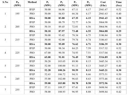
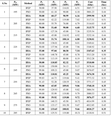
The standard 6-bus system is composed of three thermal generating units and three load buses. The cost curve data is presented in G. Ravi et al. [13]. The line parameters are as given in Wood and Wollenberg [12]. This 6-bus test system supplies ten different heuristically taken load demands with load pattern as given in [13]. The solution of ELD problem without and with valve point effect is shown in the Table.1 & 2. It is observed that the proposed HSA method is better than the other methods in saving the cost of generation considerably, reducing line losses and also reducing execution time, especially while
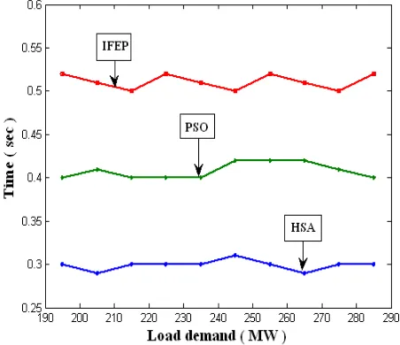
[image:3.612.326.559.102.295.2]considering the valve point loading effect. The execution time of HSA is almost constant for all level of loads shown in Fig.2 & 3.
Fig. 1 Convergence characteristic (magnified up to 100 iterations) of 6 bus system with valve point loading effect
4.2
Test System 2
[image:3.612.325.551.485.680.2]29
Fig. 2 Comparison of execution time of 6-bus systemwithout valve point loading
Fig. 3 Comparison of execution time of 6-bus system with valve point loading
4.3
Test System 3
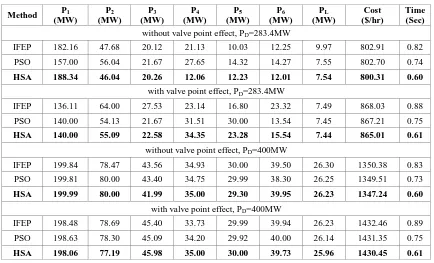
[image:4.612.94.521.375.696.2]To verify further the effectiveness of the proposed HSA approach, the IEEE-30 bus system was taken which composed of six thermal generating units. The cost curve data is presented in G. Ravi et al. [13] and all other necessary information is presented in Lee et al. [15]. Due to the lack of space, only two load patterns of the system are shown in Table.5. The corresponding simulation results of IFEP, PSO and the proposed HSA method are given in Table.6 for 283.4 MW and for 400MW load demands. It is clearly seen that the considerable saving in generation cost could be obtained by HSA method when compared to the other two methods. Furthermore it is observed that, the line losses are also reduced, the execution time is also less and almost constant. In all the test cases, it is observed that due to the presence of valve point effect, the cost of the system with valve point loading is more than the system without valve point loading.
Table. 1 Comparative result of standard 6-bus system without valve point effect
S.No PD (MW)
Method P1
(MW)
P2 (MW)
P3 (MW)
PL (MW)
Cost ($/hr)
Time (Sec)
1 195
IFEP 50.00 84.06 67.11 6.17 2941.67 0.52
PSO 50.00 84.83 66.34 6.17 2941.63 0.40
HSA 50.00 83.80 67.35 6.15 2941.43 0.30
2 205
IFEP 50.00 88.79 72.77 6.56 3064.98 0.51
PSO 50.10 89.45 72.01 6.56 3064.96 0.41
HSA 50.10 87.97 73.48 6.55 3064.88 0.29
3 215
IFEP 50.00 93.42 78.34 6.75 3186.84 0.50
PSO 50.00 92.00 79.74 6.74 3186.65 0.40
HSA 50.00 95.09 76.62 6.71 3186.39 0.30
4 225
IFEP 50.00 98.34 84.25 7.59 3317.32 0.52
PSO 67.00 90.58 74.93 7.51 3317.04 0.40
HSA 65.00 91.01 76.49 7.50 3316.89 0.30
5 235
IFEP 50.20 103.05 89.90 8.15 3445.34 0.51
PSO 52.00 100.00 91.13 8.13 3445.27 0.40
HSA 52.28 100.26 90.59 8.13 3445.21 0.30
6
245
IFEP 52.63 106.72 94.31 8.66 3573.51 0.50
PSO 55.00 102.00 96.63 8.63 3573.46 0.42
HSA 59.00 103.80 90.78 8.58 3572.96 0.31
7 255 IFEP 57.11 109.37 97.41 8.89 3698.94 0.52
30
Table. 2
Comparative result of standard 6-bus system with valve point effect
HSA 60.41 107.97 95.48 8.86 3698.65 0.30
8 265
IFEP 61.57 112.10 100.75 9.42 3828.51 0.51
PSO 62.00 111.90 100.52 9.42 3828.46 0.42
HSA 65.75 110.54 98.10 9.39 3828.19 0.29
9 275
IFEP 65.94 114.70 103.81 9.45 3952.28 0.50
PSO 68.00 113.73 102.71 9.44 3952.23 0.41
HSA 68.02 112.98 103.43 9.43 3952.13 0.30
10 285
IFEP 70.47 117.38 107.19 10.04 4083.60 0.52
PSO 72.00 116.73 106.31 10.04 4083.57 0.40
HSA 72.02 116.41 106.60 10.03 4083.51 0.30
S.No PD
(MW) Method
P1 (MW)
P2 (MW)
P3 (MW)
PL (MW)
Cost ($/hr)
Time (Sec)
1 195
IFEP 50.00 37.50 114.01 6.51 3007.77 0.50
PSO 50.00 61.18 90.00 6.18 3001.23 0.44
HSA 50.00 60.17 90.99 6.16 2999.90 0.35
2 205
IFEP 50.00 42.22 119.80 7.02 3117.31 0.51
PSO 80.00 55.79 76.00 6.79 3116.03 0.45
HSA 70.00 51.68 90.00 6.68 3115.75 0.35
3 215
IFEP 50.00 127.36 45.00 7.36 3235.54 0.51
PSO 60.00 45.00 116.92 6.92 3232.16 0.44
HSA 70.00 51.74 100.14 6.88 3230.01 0.35
4 225
IFEP 50.00 138.01 45.00 8.01 3349.61 0.51
PSO 50.00 137.96 45.00 7.96 3348.92 0.45
HSA 55.00 97.04 80.50 7.54 3347.63 0.35
5 235
IFEP 50.00 148.78 45.00 8.78 3513.20 0.50
PSO 50.00 113.19 80.00 8.19 3512.28 0.45
HSA 50.00 110.85 82.32 8.17 3510.00 0.35
6
245
IFEP 50.00 150.00 54.13 9.13 3678.44 0.50
PSO 99.86 109.21 45.00 9.07 3676.07 0.45
HSA 98.00 110.81 45.25 9.06 3674.30 0.35
7 255
IFEP 99.83 44.73 119.84 9.41 3773.32 0.51
PSO 91.43 52.28 120.55 9.26 3771.17 0.45
HSA 90.00 65.05 109.01 9.06 3768.18 0.35
8 265
IFEP 99.89 129.93 45.00 9.82 3884.54 0.50
PSO 99.00 55.99 119.80 9.79 3880.53 0.45
HSA 95.00 59.92 119.80 9.72 3876.57 0.35
9 275
IFEP 99.88 140.33 45.50 10.72 4014.99 0.50
PSO 50.00 133.17 101.50 9.67 4012.85 0.45
HSA 51.00 133.65 100.01 9.66 4010.27 0.35
31
Table. 3 Heuristic Load Pattern for IEEE-14 bus systemPD (MW)
Bus. No
Load (MW)
Bus. No
Load (MW)
Bus. No
Load (MW)
Bus. No
Load (MW)
Bus. No
Load (MW)
289
1 0 4 47.80 7 0 10 09.00 13 13.50
2 21.70 5 07.60 8 30.00 11 03.50 14 14.90
3 94.20 6 11.20 9 29.50 12 06.10
260.01
1 0 4 43.02 7 0 10 08.10 13 12.15
2 27.00 5 06.84 8 84.78 11 03.15 14 13.41
3 19.44 6 10.08 9 26.55 12 05.49
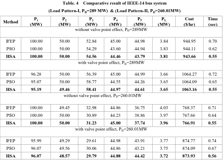
Table. 4 Comparative result of IEEE-14 bus system
(Load Pattern-I, PD=289 MW) & (Load Pattern-II, PD=260.01MW)
Method P1 (MW)
P2 (MW)
P3 (MW)
P4 (MW)
P5 (MW)
PL (MW)
Cost ($/hr)
Time (sec) without valve point effect, PD=289MW
IFEP 100.00 50.00 52.84 45.00 44.98 3.84 944.95 0.70
PSO 100.00 50.00 54.29 43.60 44.94 3.83 944.11 0.62
HSA 100.00 50.00 54.56 44.46 43.79 3.81 943.66 0.55
with valve point effect, PD=289MW
IFEP 96.28 50.00 56.39 45.00 44.99 3.66 1064.27 0.72
PSO 95.07 50.00 58.77 44.55 44.26 3.65 1064.09 0.65
HSA 95.19 49.46 58.41 44.97 44.61 3.65 1063.16 0.55
without valve point effect, PD=260.01MW
IFEP 100.00 49.45 32.98 44.86 36.75 4.03 768.37 0.71
PSO 100.00 50.00 30.89 44.23 38.86 3.97 767.66 0.64
HSA 100.00 50.00 31.23 45.00 37.74 3.96 766.91 0.55
with valve point effect, PD=260.01MW
IFEP 95.99 49.29 29.61 44.98 43.91 3.77 874.77 0.74
PSO 96.07 49.56 30.06 44.86 43.21 3.75 874.09 0.67
[image:6.612.81.519.265.580.2]HSA 96.07 48.57 29.79 44.88 44.42 3.72 873.93 0.56
Table. 5 Heuristic Load Pattern for IEEE-30 bus system
PD (MW)
Bus. No
Load (MW)
Bus. No
Load (MW)
Bus. No
Load (MW)
Bus. No
Load (MW)
Bus. No
Load (MW)
283.4
1 0 7 22.80 13 0 19 9.50 25 0
2 21.70 8 30.00 14 6.20 20 2.20 26 3.50
3 2.40 9 0 15 8.20 21 17.50 27 0
4 7.60 10 5.80 16 3.50 22 0 28 0
5 94.20 11 0 17 9.00 23 3.20 29 2.40
PSO 52.00 131.27 112.00 10.27 4116.16 0.45
32
6 0 12 11.20 18 3.20 24 8.70 30 10.60
400
1 0 7 22.80 13 33.50 19 9.50 25 0
2 84.20 8 30.00 14 6.50 20 12.20 26 0
3 12.40 9 0 15 8.50 21 17.50 27 0
4 7.60 10 15.80 16 13.50 22 0 28 0
5 41.70 11 0 17 9.00 23 3.20 29 22.40
[image:7.612.90.524.233.496.2]6 0 12 27.30 18 3.10 24 8.70 30 10.60
Table. 6 Comparative result of IEEE-30 bus system
(Load Pattern-I, PD=283.4 MW) & (Load Pattern-II, PD=400MW)
5.
CONCLUSION
This study was done on the application feasibility of harmony search algorithm for solving economic load dispatch by taking into account of load pattern problem. The simulation result shows that the proposed method can give competitively cheaper generation cost and also considerable reduction in the transmission line losses, Further more the execution time for all the three test systems under consideration are almost constant and less when compared to the IFEP & PSO methods. Hence, the performance of the proposed HSA appears to be an efficient and powerful tool to solve highly nonlinear discontinuous cost functions of ELD problem and to obtain globally better optimum solution. The future work will be explored to incorporate the ramp rate and multi-fueling options constraints into the objective function formulation by using the proposed HSA technique.
6.
ACKNOWLEDGMENTS
The assistance and suggestions of Dr. Zong Woo Geem is kindly acknowledged.
7.
REFERENCES
[1] D. C. Walter, and G. B. Sheble, “Genetic algorithm solution of economic dispatch with valve point loading, ”IEEE Trans. Power Systems, vol.8, no.3, pp.1325–1331, Aug1993.
[2] K. P. Wong, and C. C. Fung, “Simulated annealing based economic dispatch algorithm,” IEE Proc. Part C, vol. 140, no.6, pp. 544–550, 1993.
[3] N.Sinha, R. Chakrabarti, and P. K. Chattopadhyay, “Evolutionary programming techniques for economic load Method P1
(MW)
P2 (MW)
P3 (MW)
P4 (MW)
P5 (MW)
P6 (MW)
PL (MW)
Cost ($/hr)
Time (Sec) without valve point effect, PD=283.4MW
IFEP 182.16 47.68 20.12 21.13 10.03 12.25 9.97 802.91 0.82 PSO 157.00 56.04 21.67 27.65 14.32 14.27 7.55 802.70 0.74
HSA 188.34 46.04 20.26 12.06 12.23 12.01 7.54 800.31 0.60
with valve point effect, PD=283.4MW
IFEP 136.11 64.00 27.53 23.14 16.80 23.32 7.49 868.03 0.88 PSO 140.00 54.13 21.67 31.51 30.00 13.54 7.45 867.21 0.75
HSA 140.00 55.09 22.58 34.35 23.28 15.54 7.44 865.01 0.61
without valve point effect, PD=400MW
IFEP 199.84 78.47 43.56 34.93 30.00 39.50 26.30 1350.38 0.83 PSO 199.81 80.00 43.40 34.75 29.99 38.30 26.25 1349.51 0.73 HSA 199.99 80.00 41.99 35.00 29.30 39.95 26.23 1347.24 0.60
with valve point effect, PD=400MW
33
dispatch, ” IEEE Transactions on Evolutionary Computation,vol.3, no.7, pp. 83–94, Feb2003.
[4] N.Sinha, R.Chakrabarti, and P.K. Chattopadhyay, “Fast evolutionary programming techniques for short term hydro thermal scheduling, ”Elect Power Syst Res, vol.6, no.2, pp 97– 103, August2003.
[5] K. P. Wong, and Y. W. Wong, “Thermal generator scheduling using hybrid genetic / simulated annealing approach, ” IEE Proc., Part C, vol.142, no.4, pp.372–380, July 1995.
[6] Lin VM, Cheng FS, and Tsay MT, “An improved tabu search for economic dispatch with multiple minima, ” IEEE Trans Power Syst, vol.17,no.1, pp 108-112, Feb2002.
[7] Park J.B, Lee K-S, Shin J-R, and Lee KY, “A particle swarm optimization for economic dispatch with non-smooth cost functions, ”IEEE Trans Power Systems, vol.20, no.1, pp. 34-42, 2005.
[8] Noman N, and Iba H, “Differential evolution for economic load dispatch problems, ” Electr Power Syst Res, vol.78 , pp.1322-1331,Nov2008.
[9] Zong Woo Geem (Ed), Music-Inspired Harmony Search Algorithm-Theory and Applications, Springer-Verlag Berlin Heidelberg, 2009.
[10] Geem ZW, Kim JH, and Loganathan, GV, “A new heuristic optimization algorithm: harmony search, Simulation, ” vol.76, no.2, pp 60–68, 2001.
[11] Lee KS, Geem ZW, “A new structural optimization method based on the harmony search algorithm, ”Comput Struct, vol.82, no.9-10, pp.781-798, Jan2004.
[12] A. J. Wood, and B. F. Wollenberg, Power Generation, Operation, and Control, New York, John Wiley & Sons, 1996. [13] G.Ravi, R.Chakrabarti, and S.Choudhuri, “Nonconvex economic dispatch with heuristic load patterns using improved fast evolutionary program, ” Elect Power Comp and Syst, vol.34, pp.37-45, 2006.
[14] V. C. Ramesh and X. Li, “A fuzzy multi objective approach to contingency constrained OPF, ” IEEE Transactions on Power Systems, vol.2, no.3, pp 1348–1354, August1997.
[15] K. Y. Lee, Y. M. Park, and J. L. Ortiz, “A unified approach to optimal real and reactive power dispatch, ”IEEE Transactions on Power Apparatus and Systems, vol.104, no.5, pp.1147-1153, May1985.
BIOGRAPHIES
R. Arul received B.E degree in Electrical and Electronics Engineering and M.E degree in Power Systems from Annamalai University in 1995, 1997 respectively. Currently, pursuing Ph.D in Annamalai University, Annamalai Nagar, Chidambaram. His research area includes electrical machines, power system operation, planning, optimization and soft computing techniques.
G. Ravi received B.E degree in Electrical & Electronics Engineering from Mysore University in 1992. M.E from Annamalai University in 1994 and Ph.D (Engg) from Jadavpur University in 2005. At present he is a faculty in Electrical & Electronics Engineering department at Pondicherry Engineering College, Puducherry. His research area includes electrical machines, power system operation, planning, optimization and soft computing techniques.