Design of Sub Arterial Urban Road using MXROAD Software

(1)

DESIGN OF SUB-ARTERIAL URBAN ROAD USING MXROAD SOFTWARE

Ali Ashraf

1

_{, Nishant Singh}

2

_{, Yashraj Shrivastava}

3

_{, JS Vishwas}

4

1,2,3

_{Student, Pes University, Bengaluru, India}

4

_{Assistant Professor, Pes University, India}

---*---Abstract –**

The project is about Design of Urban Road using MXROAD Software and is done for a stretch of 1.51 km from Devegowda Circle to Nice Road via Kerekodi Road. The intention of this study is to import road design into the software as well as relate with design standards applied into the software. To know the existing condition of the road cross sectional elements, road inventory is done. Survey data is extracted from GIS i.e., Google Earth and road design is done using MXROAD software which is an advance string base tool that enables rapid designing of all road type with accuracy. In road design, geometric design which consists of alignment (both horizontal and vertical), carriageway, super elevation and extra widening along with road cross sectional elements which consists of shoulder, kerbs, verges and footpath followed design standard as per IRC: 86-1983. Earthwork is done in such a way that the cut and fill percent gets roughly matched. The flexible pavement design is carried out as per IRC: 37-2012 and for that traffic volume survey and CBR test is done. A detailed report of each segment is generated with great ease using MXROAD. As 27 km of road is build each day in India. So, adopting software in this practice will optimize accuracy and safety while minimizing the cost and time.

Key Words:

MXROAD, Google Earth, Geometric Design, Flexible Pavement, Traffic Volume Survey, CBR Test

1. INTRODUCTION

Bengaluru is home to 2nd_{highest number of vehicle in India}

having vehicle population of about 8.4 million [1]. Statistics says that the number has more than doubled in the past 10 years, with the addition of 4 million new vehicles. There are 4.86 million two wheelers and 1.35 million four wheelers. BMTC provides transport facilities to over 5 million commuters. These buses depend on urban roads which are maintained by BBMP to carry out these populations.Total area of Bengaluru covers 741 sq.km and road length of 13000 km, increment of 1,254 percent from 1976. Roads are just developed over time but no improvements were done in order to ensure safe pedestrian traffic and non motorized facility. So, a sub arterial road is selected from a place where population of both vehicle and people has seen an enormous growth. Since growth was not planned, transport planning was also not controlled.

1.1 Project Location

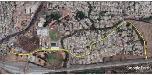
The stretch selected is 1.51 km and is from Devegowda Circle to NiceRoad via Kerekodi Road.As it covers shortest distance and connects outer ring road traffic to Raja Rajeshwari Nagar in the right via Legacy Road which makes it an

[image:1.595.309.559.301.424.2]

important road.At the start of road up to 100m there are lots of shops and pedestrian traffic is high and PES University back gate is 400m from starting point. At 600m the road is connected to legacy road which creates three way intersection over there. From that three way intersection to Hayagreeva Temple, it is 600m. And there are residential area on both side of the road.From Hayagreeva Temple till the end of the stretch , there is low line area on the right and Hosakerehalli Lake on the left which 59.25 acre in the area where recently Chola structure is found.

Fig -1:

Existing site location

1.2 MXROAD Software

(2)

designed and controlled by MXROAD software. Earth work calculation and pavement design are also carried out and done to high accuracy by using MXROAD.

1.3 Project Objectives

 Road inventory to know the existing condition of road.

 Producing proper horizontal and vertical alignment.

 Providing proper carriageway, shoulder, kerbs, verges or footways wherever required based on IRC.

 Providing widening wherever required.

 Introducing super elevation on curves.

 Cut and fill data extraction based on earth work.

 Traffic Volume survey.

[image:2.595.354.549.80.166.2]

 Pavement design based on CBR value and average daily traffic.

Fig -2: Flow chart of methodology

2. Field and Laboratory Investigation

In this project following surveys is conducted as listed below.

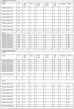
[image:2.595.340.551.305.439.2]

2.1 Collection of 4 Soil sample from 350m each.

Fig -3:

Collection of soil sample

2.2 Road inventory

[image:2.595.41.284.337.619.2]

In this road inventory length of road is measured along with the land used and terrain up to that particular length. Road component like width of the carriageway and shoulder along with its present condition and type is checked.

Table -1: Summary of road inventory

Geometric features Project Road

Length 1510 m

Width 6.92 m

Number of lanes Two lane

Traffic movement 2-way

Divided/undivided Undivided

Shoulder type Unpaved

Pavement drainage condition Poor

Road side drainage Poor

Land use Commercial & Residential

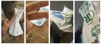
2.3 Traffic volume survey

Traffic volume is defined as number of vehicles crossing a section of road per unit time at any particular period. It is conducted to collect data on number of vehicles or pedestrians that pass a point on a road facility during a specified time period.

 Average daily traffic

We calculated the average daily traffic for a design of pavement. For design of pavement only number of commercial vehicles i.e., vehicles of gross weight of 30 KN or more will be considered [3]. For the design of two lane single carriageway road, the design should be based on 50 percent of total number of commercial vehicle in both directions [3].

According to equation [5],

(3)

[image:3.595.28.322.107.535.2]

Table -2: Number of commercial vehicle

No. of Commercial Vehicle in both

the direction for peak hour = 241 + 251 = 492 50% of the above value = 246

Average daily traffic = 2460 vehicle/day

2.4 Laboratory investigations

In the evaluation level laboratory description is an important feature. This would help in the field at the time of construction to know the properties of materials. For road construction works, properties of soil at subgrade level are required to be known. Soil testing is done in the laboratory as per IRC-37-2012. The laboratory tests that were conducted on soil samples are :

Table -3: Determination of OMC

Chart -1: Moisture Content vs Dry Density

OMC = 10.3%

MDD = 2.11 kN/m3.

 California Bearing Ratio MORNING PEAK HOUR

A to B

Time Car Mini

Bus Bus 2-Axle Truck 3-axle Truck JCB 3dx Tracktor Total

08:30 to 08:45 am 38 2 3 3 2 0 0 48

08:45 to 09:00 am 48 2 2 4 2 0 2 60

09:00 to 09:15 am 58 1 1 2 1 0 0 63

09:15 to 09:30 am 43 1 1 2 0 0 0 47

09:30 to 09:45 am 46 0 2 5 1 0 0 54

09:45 to 10:00 am 42 2 2 3 1 0 0 50

10:00 to 10:15 am 47 4 1 1 2 0 1 56

10:15 to 10:30 am 56 1 2 1 2 0 0 62

B to A

08:30 to 08:45 am 54 3 1 6 0 0 0 64

08:45 to 09:00 am 58 1 1 1 0 0 0 61

09:00 to 09:15 am 43 3 0 4 0 0 0 50

09:15 to 09:30 am 52 0 3 1 0 0 0 56

09:30 to 09:45 am 58 0 3 1 2 0 1 65

09:45 to 10:00 am 49 5 2 4 0 0 0 60

10:00 to 10:15 am 53 1 0 2 0 0 1 57

10:15 to 10:30 am 37 2 1 1 0 0 1 42

EVENING PEAK HOUR A to B

Time Car Mini

Bus Bus 2-Axle Truck 3-axle Truck JCB 3dx Tracktor Total

05:30 to 05:45 pm 25 0 0 0 0 0 0 25

05:45 to 06:00 pm 27 1 0 0 0 0 0 28

06:00 to 06:15 pm 21 0 1 2 0 0 0 24

06:15 to 06:30 pm 31 3 0 1 1 0 0 36

06:30 to 06:45 pm 25 0 2 0 0 0 0 27

06:45 to 07:00 pm 23 1 1 1 1 0 0 27

07:00 to 07:15 pm 28 1 1 1 0 0 0 31

07:15 to 07:30 pm 32 1 0 1 0 0 0 34

B to A

05:30 to 05:45 pm 48 2 2 4 0 1 0 57

05:45 to 06:00 pm 33 0 1 0 0 0 0 34

06:00 to 06:15 pm 35 0 1 0 2 0 0 38

06:15 to 06:30 pm 29 1 0 3 0 0 1 34

06:30 to 06:45 pm 34 2 1 1 1 0 0 39

06:45 to 07:00 pm 36 0 0 0 0 1 0 37

07:00 to 07:15 pm 30 1 0 1 0 0 0 32

07:15 to 07:30 pm 31 1 1 0 1 0 0 34

Sl No. Particulars Unit Mould 1 Mould 2

Determination of Bulk Density of Soil

1 Volume of mould cm3 1001.38 1001.38 2 Weight of Empty

Mould gm 1992 1992 3 Weight of Mould

+ Compacted Soil gm 4374 4368 4 Weight of

Compacted Soil gm 2387 2376 5 Weight Density

(w/v) gm/cm3 2.376 2.376

Sl No. Particulars Unit Mould 1 Mould 2

Determination of Moisture Content and Dry Density of Soil

1 Cup Number 7-1 5-3 2 Weight of Empty

Cup gm 23.4 23.5 3 Weight of Cup +

Wet Soil gm 29.4 30.3 4 Weight of Cup +

Dry Soil gm 28.8 30.2 5 Weight of Dry

Soil gm 5.4 6.7 6 Moisture

[image:3.595.346.563.112.566.2]

(4)

[image:4.595.113.235.77.186.2]

Fig -4: Making of Mould and taking reading from CBR

[image:4.595.51.286.261.576.2]

reading

Table -4: Proving Ring Road

Penetration

(mm) Proving Ring Mould 1 Mould 2 Average

Reading

Proving Ring Reading

0.0 0 0 0

0.5 5 4 5

1.0 10 9 10

1.5 15 13 14

2.0 18 14 16

2.5 20 18 19

3.0 22 20 21

4.0 25 23 24

5.0 32 30 31

7.5 37 42 40

10.0 39 52 46

12.0 54 46 50

Chart -2: Penetration vs PRR Graph

From the Above Figure

PRR Load CBR

At 2.5 mm Penetration

19 106 8%

3. Design Proposal

3.1 Importing Survey Data from Google Earth to MXROAD

[image:4.595.319.525.275.488.2]

3.1.1 Creating path in Google earth

Fig -5: Creating path in Google earth

3.1.2 Adding Elevation Using GPS visualizer

 Open gpsvisualizer.com and add elevation

 File can be downloaded in gpx format

Fig -5: Adding Elevtion

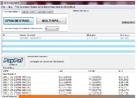
[image:4.595.325.545.545.702.2]

3.1.3 Changing gpx to csv format using TCX convertor

(5)

[image:5.595.49.275.113.234.2]

3.1.4 Converting Latitude, Longitude to Northing and Easting using UTM convertor

Fig -7: Changing GEO Coordinates to UTM

After that in csv file string name of centerline is included and by using ASCII import command, it is imported.

[image:5.595.359.509.221.354.2]

Fig -8: Northing, Easting, Elevation &String name

3.2 Geometric design using MXROAD

3.2.1 Sight distance

For Sub-arterial road [4], Design speed = 60 km/h So, SSD = 80m

As road is dual lane single carriageway, ISD = 2*SSD = 160m

By using equation,

OSD = 0.28Vbt + 0.28VbT + 2S + 0.28VT

OSD = 376m

3.2.2 Horizontal alignment

Radius of curve, r = V2_/127(e+f)

Minimum radius = 40m Maximum radius = 150m

Fig -9: Parameters in Horizontal Alignment

3.2.3 Vertical Alignment

From page no. 23[4],

Maximum grade % for urban road = 4% Minimum grade % for urban road = 0.5% From Exhibit 3-77[6],

Hog curve K value = 195 From Exhibit 3-79[6], Sag curve k value = 18

Minimum Length of vertical curve = 40m(From Table 14[4])

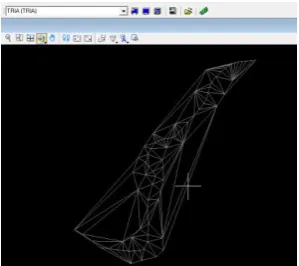
Fig -10: Traingulation model

Fig -11: Parameters in Vertical alignment

Creating Vertical Alignment using Add IP mode:

Fig -12: Add IP mode

3.2.4 Carriageway

From Table 5[4], Width of Carriageway 2- Lane with Kerbs = 7.50m

Camber should be between 1.7 – 3.0 % In urban roads of Bengaluru = 2%

(6)

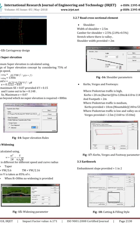
Fig -13: Carriageway design

3.2.5 Super elevation

Maximum Super elevation is calculated using,

Design of Super elevation concept by considering 75% of design speed,

R ruling =

R ruling = 130m

And e =

e = 0.1222 > 0.07

So, maximum SE = 0.07 provided if f < 0.15 and f came out to be = 0.148 .

So, Maximum e = 0.07

[image:6.595.56.541.26.805.2]

Radius beyond which no super elevation is required = 800m

Fig -14: Super elevation Rules

3.2.6 Widening

It is calculated using,

So, it is different for different speed and curve radius

 Taper

TD = VW/3.6 TM = VW/2.16 where V is taken as 85% of v.

[image:6.595.68.256.380.486.2]

 When R>300m no widening is provided

Fig -15: Widening parameter

3.2.7 Road cross sectional element

 Shoulder:

Width of shoulder = 2.5m

Camber for shoulder = 2.5% (2.0%+0.5%) Stretch where there is valley ,

Shoulder width provided = 2m

Fig -16: Shoulder parameters

 Kerbs, Verges and Footways:

Where Pedestrian traffic is high,

Kerbs = 20 cm (Barrier)(0 to 120m & 610 to 1140m) And Footpath = 2m

Where Pedestrian traffic is medium,

[image:6.595.366.536.440.544.2]

Kerbs provided = 10cm (Mountable)(140 to 530m) Where Pedestrian traffic is low and valley on side, Verges provided = 2.5m (1160 to 1510m)

Fig -17: Kerbs, Verges and Footway parameter

3.3 Earthwork

Embankment slope provided = 1 in 2

Fig -18: Cutting & Filling Style 2

(0.278 ) / (V g ef)

2 (0.75*0.278* ) /V gR

2

2 9.5

nl V

w

R R

[image:6.595.359.523.622.740.2]

(7)

3.4 Pavement design

Traffic in msa,

N = 55.66 msa And CBR is taken as = 8% As per Chart given in Page 27 [3], Binder Course = 41 mm

Dense Bituminous Macadam = 102 mm Granular Base = 250 mm

[image:7.595.32.555.40.805.2]

Granular Sub Base = 200 mm

Fig -19: Pavement Design Parameters

[image:7.595.328.539.61.581.2]

4. Output from Software

 Horizontal Alignment

[image:7.595.83.255.256.362.2]

Fig -20: Horizontal Alignment Preview

Table -5: Horizontal Report Curve 1

Horizontal Alignment Report

Model: DESIGN String: MC00 Units: Metric

Date: 16/04/2018 at 10:48:07 AM ********Element 1 Straight********

Bearing 77 59 33.866 Length 25.619 ********Transition********

Long Tangent 12.073 Short Tangent 6.032

Chord Bearing 79 38 13.695 Chord Length 18.076 Transition Start X 774751.651 Transition Start Y 1430543.108

Transition End X 774769.433

Transition End Y 1430546.359 ********Element 2 Arc********

Chord Length .706 Radius 105.000 Chord Bearing 83 07 08.295

Arc Length .706

Tangent .353 Included Angle 00 23 07.655

********Transition******** Long Tangent 12.073

Short Tangent 6.032 Chord Bearing 86 36 02.894

Chord Length 18.076 Transition Start X 774770.134 Transition Start Y 1430546.444

Transition End X 774788.178 Transition End Y 1430547.516

[image:7.595.58.246.418.547.2]

 Vertical Alignment

Fig -21: Vertical Alignment Preview

Table -6: Vertical Alignment Report Curve 1

Vertical Alignment Report

Model: DESIGN String: MC00 Units: Metric

Date: 16/04/2018 at 10:55:32 AM ********Element 1 Grade********

Gradient -.765 Gradient Length 210.218 Begin on Gradient Chainage

0+000.000

Begin on Gradient Level 831.602 Gradient End Chainage 0+210.218

Gradient End Level 829.994 ********Element 2 Vertical

365((1 ) 1) * * *

n

r

N A D F

r

(8)

Curve******** Algebraic Difference .142 Curve Start Gradient -.765 Curve End Gradient -.623

Curve Length 2.549 K Value 18.000 Curve Type Sag Vertical Radius 1799.995 Curve Start Chainage 0+210.218

Curve Start Level 829.994 Curve End Chainage 0+212.767

Curve End Level 829.976

[image:8.595.39.536.53.758.2]

 Super elevation

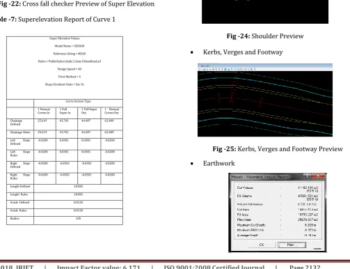
[image:8.595.51.279.66.392.2]

Fig -22: Cross fall checker Preview of Super Elevation

Table -7: Superelevation Report of Curve 1

 Extra Widening

For Curve 1, We = 0.86

TD = 10.15 TM = 16.92

Fig -23: Widening Preview

[image:8.595.52.556.404.790.2]

 Shoulder

Fig -24: Shoulder Preview

 Kerbs, Verges and Footway

Fig -25: Kerbs, Verges and Footway Preview

 Earthwork

Super Elevation Values Model Name = DESIGN Reference String = MC00 Rules = PublicStyles\India 2-lane UrbanRoad.srl

Design Speed = 60 Pivot Method = 4 Slope/Gradient Units = Dec %

Curve Section Type 1 Normal

Crown In 1 Full Super In 1 Full Super Out 1 Normal Crown Out Chainage

Defined 25.619 43.701 44.407 62.489 Chainage Rules 25.619 43.701 44.407 62.489 Left Slope

Defined -0.0200 0.0381 0.0381 -0.0200 Left Slope

Rules -0.0200 0.0381 0.0381 -0.0200 Right Slope

Defined -0.0200 -0.0381 -0.0381 -0.0200 Right Slope

Rules -0.0200 -0.0381 -0.0381 -0.0200 Length Defined 18.082

Length Rules 18.082 Grade Defined 0.0120 Grade Rules 0.0120

[image:8.595.61.230.453.728.2]

(9)

[image:9.595.39.287.230.433.2]

Fig -26: Earthwork Result

Fig -27: Earthwork Preview

[image:9.595.32.560.488.793.2]

 Pavement Design

[image:9.595.40.311.490.758.2]

Fig -28: Pavement Design Parameter

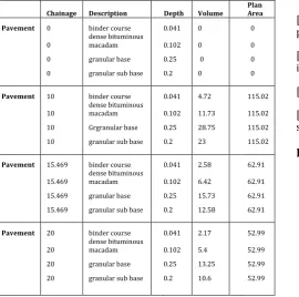
Table -8: Pavement Design Report for 0 to 20 Chainage

Chainage Description Depth Volume Plan Area

Pavement 0 binder course 0.041 0 0 0

dense bituminous

macadam 0.102 0 0 0 granular base 0.25 0 0 0 granular sub base 0.2 0 0

Pavement 10 binder course 0.041 4.72 115.02 10 dense bituminous macadam 0.102 11.73 115.02 10 Grgranular base 0.25 28.75 115.02 10 granular sub base 0.2 23 115.02

Pavement 15.469 binder course 0.041 2.58 62.91 15.469

dense bituminous

macadam 0.102 6.42 62.91 15.469 granular base 0.25 15.73 62.91 15.469 granular sub base 0.2 12.58 62.91

Pavement 20 binder course 0.041 2.17 52.99 20 dense bituminous macadam 0.102 5.4 52.99 20 granular base 0.25 13.25 52.99 20 granular sub base 0.2 10.6 52.99

5. CONCLUSIONS

 The proposed alignment is designed to match with the existing alignment but got some deviation considering IRC value.

 Design speed are formulated for ruling design speed of 60 km/h and minimum design of 30 km/h.

 Alignment proposed encounters minimum horizontal curve radius of 40m at two junction where speed is restricted to minimum.

 To increase the driver’s and passenger’s comfort ability on each curve, super elevation up to 7% and widening up to 1.43 m is suggested.

 High design precision along with rapid designing of the road is achieved by MXROAD.

ACKNOWLEDGEMENT

We will like to acknowledge Prof. BV Ramesh, Assistant professor, Department of Civil Engineering, PES University, Bengaluru, Karnataka, India for his constant support and guidance during the project.

REFERENCES

[1] Part XII-A, Series-30, Directorate of census operations, Karnataka, Census of India 2011
[2]“https://timesofindia.indiatimes.com/city/Bengaluru/nu mber-of-vehicles-in-bengaluru-more-than-doubles-70lakh-in-10years/articleshow/60445744.cms”
[3] IRC-37-2012, “Guidelines for the design of flexible pavement”.
[4] IRC-86-1983, “Geometric design standard for urban roads in plains”.
[5] IRC-9-1972, “Traffic census on Non urban roads”
[6] AASHTO A policy on geometric design of highway and streets (Green book, 2011 edition)
BIOGRAPHIES
Ali Ashraf has creative approach
© 2018, IRJET | Impact Factor value: 6.171 | ISO 9001:2008 Certified Journal | Page 2134
Nishant Singh has critical thinking
skills. He aims to work in Civil Engineering industry particularly in Transport and Communication infrastructure.
Yashraj Shrivastava has excellent
communication skills and decision making abilities. He aims to be a Construction Estimator for cost effective budgeting of project.
J S Vishwas Assistant Professor in
Department of Civil Engineering, Pes University, Bengaluru, India. He is life time member in in International Society of
Research Development and Institution of Highway Engineers. He is also a board of