Relevance of An Accuracy Control
Module - Implementation into An
Economic Modelling Software
Buda, Rodolphe
GAMA - Université de Paris 10 Nanterre
2005
Online at
https://mpra.ub.uni-muenchen.de/36520/
Implementation into An Economic Modelling
Software
Rodolphe BUDA
GAMA, University of Paris 10
2005
——————————————————————————————–
Summary
Economic modelers or econometricians know that they have to control the accuracy of the computations, to get their results safe. Unfortunately, even if a few softwares allow to control it (especially in using an interval arith-metic), most of them are presented like black boxes, from an arithmetical point of view. We have tried, in this paper, to provide the point of view of a macroeconomic modelling software’s builder. After having recalled the accu-racy problem and its solutions (algebraic and arithmetical), we’ll present the
GNOMBR software we have developed, based on multiple precision arithmetic methods. Then we’ll present an application to an input-output model. Then we’ll give elements to conclude to the relevance of this technique.
Key-words : Modelling software - Floating point arithmetic - Accuracy re-sults control - Arithmetic accuracy computer
J.E.L. Classification: C82, C87, C88.
0. - Introduction
This paper collects the reflections we have had during the building
of a multi-dimensional1 economic modelling software (SIMUL i.e. Système
Intégré de Modélisation mULtidimensionnelle)2. This software usually can
estimate multi-dimensional econometric equations quickly and solve the
whole system3. So it’s divided in some modules (estimation, data bank
ma-nagment and so on). During this work, we have had a reflection about the arithmetic accuracy trouble. Hence, we have decided to build a specific
arith-metic tool (GNOMBR i.e. Grands NOMBRes). The implementation of
ano-ther arithmetic into an economic model is not new4. However, we provide
here the double economist and software developer point of view. Furthermore, our tool is a multiple precision arithmetic implemented in Turbo-Pascal 7.0 available in two versions : library and direct Dos prompt executable version. We have divided this paper into two parts. In a first part, we’ll recall the arithmetic accuracy problem. Then we’ll present the classical solutions and the recent arithmetical substitution solutions. We’ll focus our analysis
on the GNOMBR software. We’ll especially present the implementation of it
in an input-output simplified model. Furthermore, we’ll present some results and some algorithms related to this software building. Finally, we’ll try to conclude about the usefulness of such tools, and about the economic’s domain where the arithmetic accuracy tools seem to be the more relevant.
1. - The arithmetic computer’s accuracy problem
In this first part, we’ll explain why the standard arithmetic computer
-the floating point arithmetic or IEEE-754 Standard - and even its
substi-tutes, will never completely satisfy the accuracy of computation. Indeed, we have to maximize the level of accuracy, in ordering elementary operations in the formulae (algebraic method) or to substitute the standard arithmetic computer by other arithmetics (arithmetic method).
a - The lack of representation of the floating-point arithmetic
One tells, when J. von Neumann considered the first results of the ENIAC computer, he was very disappointed because of its lack of accuracy. This problem comes from the unperfect arithmetic representation of the digits.
All computers have got this trouble5 : ordinary personal computers, super
1. - Multi-regional (r), multi-sectoral (s), multi-period (t) analysis.
2. - The building of this software is integrated in the economic thesis we are finishing, "Modélisation multi-dimensionnelle et analyse multirégionale de l’économie française" un-der the supervision of the Professeur Raymond Courbis.
3. - We only need an instruction to implement such equations :Ytr,s=X r,s
t .ar,s+ε r,s t .
computers (see eg.1) and formal computation is affected too (see eg.2).
——————————————————————————————–
#1 - The equation system6
r = 9x4−y4 + 2y3
x= 10864
y = 18817
providesr= 0 with aCDC-7600
com-puter,r= 2 with aCRAY ONE
com-puter, andr= 7.081589E+ 08 with a
VAX computer, but the exact result
isr = 1.
#2 - The series7
u0 = 2
u1 =−4
un+1 = 111− 1130un +
3000
un.un
−1
provides
u90 = 99.998040316541816165. . .
with Maple software, but the exact result is
u90= 6.0000000996842706405. . .
——————————————————————————————–
Fig.1 - Two examples of accuracy troubles during computation
The trouble comes from the unperfect computer’s arithmetic, the floating-point arithmetic. It’s impossible to represent the whole properties of the real numbers with this arithmetic, especially continuity property. According to a mathematical point of view, it’s a nonsense to actually compute a limit or a
derivation function. ∀ element X ∈ R represented by the floating element8
˜
X which belongs to F, we have
˜
X=s.M.be
wheres is the sign of ˜X,M the mantissa encoded with t digits which belong
to thebbase, andeis the exponent. Because of the finite size of the mantissa,
during calculation, the computer truncates the numbers9.
6. - From M.Pichat & J.Vignes (1993, pp.3-5).
7. - From M.Daumas & J.M.Muller (Eds.) (1997, pp.2-8).
8. - See M.La Porte & J.Vignes (1974, Algorithmiques numériques - Tome 1, Paris, Technip, 226 p. For an axiomatic presentation, see D.E.Knuth (1997, pp.229-45), especially pp.17-39.
Thus, we encounter two kinds of problems :
1˚- the computer can’t reach the infinite limits of the real numbers en-semble (the greatest positive number is 1.0E+40, but it’s not infinite10.
2˚- the computer can’t represent the separability property of numbers :
1.0E+40 + 1 = 1.0E+40. Unfortunately, a computer doesn’t follow a syste-matical rule of rounded numbers. We cant expect if truncation of the real
number will overestimate or underestimate it. Both numbers E.FFFFFF47
and E.FFFFFF54 will be truncated in E.FFFFFF5. However, the number of significantly digits follows a Laplace-Gauss statistic rule11
Furthermore, the trouble is not the same for all operators12 and
algo-rithms. M.Pichat and J.Vignes (op.cit.) have classified three cases :
1˚ - "Finish algorithms" : The solution computed should be exact. From matrix algebra computation (Gauss-elimination methods...).
2˚- "Iterative algorithms" : The solution belongs to a convergence interval. From matrix algebra computation (Gauss-Seidel, Newton methods...). The algorithm converges if F(Xq) = 0 ; stationary if |Xq−Xq−1| = 0 ; divergent
if q > Nnmax where F represents the algorithm applied to the variable X
duringq iterations, and 0 represents the data process zero, significantly near
from his mathematical value.
3˚- "Approached algorithms" : The solution depends on an interval of discretization13. From the Differential calculus.
b - The main algebraic control method
We here expose the two main algebraic control methods, which are the
Conditioning method and theHorner’s rule.
10. - We have to specify here, that until the sixties, the arithmetical representation of infinitesimal numbers were sometimes paradoxical. To correct this problem, A.Robinson (Non-Standard Analysis, North-Holland, Amsterdam, 1966), has divided R+ into three parts of numbers : the ideally little numbers (i-little), theappreciable numbers, and the
ideally great numbers(i-great) - see M.Diener & A. Deledicq,Leçon de calcul infinitésimal, Paris, A.Colin, 1989. Such innovation should provide another way of progress toward better accuracy of arithmetic computers.
11. - See M.Maillé (1982).
12. - Division operator deteriorates more the accuracy of the results than multiplication, addition or substraction.
(i) The conditioning method : Conditioning a system X.a= b means we
compute the following formula Cond(X) = √λmax
√
λmin, where λi are the
eigen-values of the matrix X, to know if the disturbance of the system during his
transformation from X.a = b to (X + ∆.X).a = (b+ ∆.b) is significant or
not. The matrix is well conditioned if Cond(X) ∼ 1 or we have to change
the pivot.
(ii) The Horner’s rule: This method14consists to change such polynomial
formulaP(x) =Pn
i=1aixi according to this way :
P(x) = an.xn+an−1.xn−1+. . . +a1.x1+a0.x0
⇒ P(x) = x(x(. . . x(anx+an−1) +. . .)) +a1) +a0
Function EVAL( P :Polynome ; X :Real ; N :Integer) : Real ; Var i :Integer ;
r :Real ; Begin
r←−P[n] ;
For i←−n-1 DownTo 0 do EVAL←−r*P[i] ; End ;
Fig.2 - Horner’s rule Algorithm
c - The arithmetic substitution methods
We can divide the search about arithmetic substitution into different kinds. The first kind keeps the basis 10 and the basic arithmetical
opera-tors and the mantissa. Other methods15 provide a greater accuracy
arith-metic. The second kind of methods changes the arithmetic and/or the basic operators.
14. - W.G.Horner presented this method in a paper in connection with a procedure for calculating the polynomial roots (Philosophical Transactions, Royal Society of London, 109, 1819, pp.308-335).
(i) The stochastic arithmetics:CESTAC16method (Contrôle etEstimation
STochatique desArrondis deCalculs) tries to estimate the number of signifi-cantly digits of a number by studying the round’s error diffusion, in evaluating the parameters of the error’s probability distribution. So, the unobservable
digits of the rounded number are simulated17.
(ii) The interval arithmetics : This method begin to check the validity
interval of the computation18, then it makes calculation on interval [a] →
[a, a] (not on numbers a) according the following operator’s rules :
Table 1 : Interval algorithm operator’s rule
Addition [a] + [b] [a+b, a+b]
Soustraction [a]−[b] [a−b, a−b]
Multiplication [a][b] [M in(ab, ab, ab, ab), M ax(ab, ab, ab, ab)]
Division [a]/[b] [a, a][1
b,
1
b] si 0∈/[b]
The lazy rational arithmetic is an alternative of the interval one. It tries
to avoid the using of rational number during computation19.
(iii) The multiple precision arithmetic : Such method involves that the
number of significant digits if very high20. Consequently, the round of the
numbers happen behind a lot of digits. The accuracy of the number in-creases. However, such arithmetic needs to implement new arithmetic
ope-rations (+−/∗ and ˆ). Multiple precision arithmetic is available in a lot of
libraries translated in languages21 and macro-languages22
16. - We could translate it with "Stochastic computation’s rounds estimation and control" - see M.Pichat & J.Vignes (1993, pp.170-175).
17. - See M.Pichat & J.Vignes,op.cit., pp.89-189 ; and M.Daumas & J.M.Muller (Eds.),
op.cit., pp.65-92)
18. - See G.Alefeld (1983). For an implementation of interval arithmetic to an input-output model, see M.E.Jerrell (1997).
19. - See M.Daumas & J.M.Muller (op.cit., pp.126-29).
20. - See R.E.Moore (1966). D.E.Knuth (op.cit., pp.265-94) and U.Kulisch (2000.a, 2000.b) (resp.) have translated this arithmetic in Assembler and Fortran (resp.). See J.Berstel et al. (op.cit., 1991, tome 2, pp.149-204) and M.Daumas & J.M.Muller (Eds.) (op.cit., pp.93-116) too.
21. - Let us quote GrandsNombres in Turbo-Pascal (J.Berstel et al.,op.cit.1991) ; MP in FORTRAN, MP GNU in C, MP FUN in C, PARI in C/C++ et RANGE en C++.
(iv) The exact arithmetic : This method computes without error neither round step. However only integer or rational numbers can be used during the
procedure. This method is unfortunately slower than the other methods23.
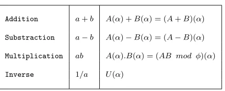
(v) The algebraic arithmetic : This method uses Bezout’s Theorem. (if A
andB are prime numbers each, (∃U, V / U.A+V.B = 1). If we consider the
polynomial relationship
A(X) = Q(X).φ(X) +R(X)
[image:8.612.164.393.315.408.2]and a=A(α) and b=B(α) hence we can define arithmetical operations24 :
Table 2 : Algebraic arithmetic operations
Addition a+b A(α) +B(α) = (A+B)(α)
Substraction a−b A(α)−B(α) = (A−B)(α)
Multiplication ab A(α).B(α) = (AB mod φ)(α)
Inverse 1/a U(α)
(vi) Dynamical arithmetic : We consider a numerical base b where we don’t use the digits {1, . . . b−1}, but the digits {−a, . . . +a} wherea / a <
b−1. For example, the number (1745)10 - read 1745 in base 10 - will be
written [2][−3][4][5] or [2][−3][4][−5]. This method (A.Avizienis, 1961) avoids to manage some carry over.
2. - Presentation of a multiple precision arithmetic tool :GNOMBR
In this second part, we firstly provide an overview of the tool, then we’ll show how we use it to program a simplified input-output model. Finally, we’ll present the basic algorithms of the tools and some significant results we can obtain with it.
a - A general presentation
We can increase the accuracy of a Turbo-Pascal program with the library of GNOMBR. GNOMBR uses the usual operators "+", "-", "*", "/" and "^", but unfortunately, it is only able to compute two operands at the same time. To compute large formulae, we have to use temporary variables and to divide it into a few formulae.
In the example on the right side, we can observe that we have computed the exponentiation by 2 of a number which has a great accuracy concerning its decimal digits.
Directly from the DOS-prompt, the GNOMBR software provides the re-sult according to his own arithme-tic and according to the floating-point arithmetic, when both computations are possible.
Each number is displayed divided into five digits packages. Each pa-ckage has got two parts : the mantissa digits and the exponent of the basis
10.
On the top of each number, accor-ding to the multiple precision arith-metics, we can find the total number of packages of the representation of the number.
CALCUL EN GRANDS NOMBRES
10 12334.0E+0005 96554.0E+0000 694.0E-0005 45647.0E-0010 54756.0E-0015 34653.0E-0020 324.0E-0025 24324.0E-0025 243.0E-0035 20000.0E-0040 ^ 2 –––––––––––––––– 19 1521.0E+0015 51374.0E+0010 87470.0E+0005 7109.0E+0000 38809.0E-0005 18440.0E-0010 88482.0E-0015 70989.0E-0020 92706.0E-0025 77532.0E-0030 18742.0E-0035 72199.0E-0040 4858.0E-0045 17764.0E-0050 63089.0E-0055 34687.0E-0060 91194.0E-0065 19146.0E-0070 24000.0E-0075
CALCUL EN VIRGULE FLOTTANTE
1.23349655400694E+0009 ^ 2
–––––––––––-1.52151374874701E+0018
The size of the accuracy depends on the memory used for the variable of the program. The accuracy indeed decreases as soon as the number and/or the size of variables increases. For only one operation, the maximal accuracy is 5000 digits. Each number is represented by some packages of five digits. For example the number1205040 becomes12.E+0005 + 5040.E+0000. The
complete software is composed of a Dos-prompt computer (CALC_GN) and an
editor (EDIT_GN). Each program gets parameters in configuration file. The
editor translates the floating-point source code in a multiple precision source code. TheTABL_GN program writes tables of results.
(i) The Dos-prompt mode computer use : The syntax is the following
CALC_GN # [Par_1][Arg_1] [Operator] [Par_2][Arg_2] [Par_3][N_file] [Com]
where # means we work directly from Dos-prompt, the Par_i are the great
numbers files used. Par_1 and Par_2 use two located codes : space bar code or "$" and,Par_3 uses two located codes :space bar code or "@" to assign an
output file, theArg_i are digital arguments (or file names) ;Com represents
a comment. Finally, theOperator is a character+ - * / or ^.
C :\>CALC_GN # 1.26636 * 65.23526 C :\>CALC_GN # $X.DAT + 65.23526 C :\>CALC_GN # $X1.DAT - $X2.DAT
C :\>CALC_GN # $X1.DAT - $X2.DAT @X1_X2.DAT
Fig.4 - Some Dos-prompt uses examples
We have presented a multiplication between1.26636et65.23526, then an addition between a number inside the X.DAT file and the number 65.23526. Then a substraction between the number inside the file X1.DAT and the
number inside X2.DAT. The result will be written in the X1_X2.DAT file.
We obtain the same results if we create an instructions file according to the same syntax25 :
~LISTE DES OPÉRATIONS ~–––––––––––––––––––– ~1.26636 * 65.23526 $X.DAT + 65.23526
$X1.DAT - $X2.DAT @X1_PL_X2.DAT CECI EST UN COMMENTAIRE
Fig.5 - Some instructions executed from a file
(ii) The program’s implementation mode use: This method is developed according to two steps26.
1˚- Firstly we have to create the Turbo-Pascal program (4.0 and the follo-wing). In this program, we have to translate each complex formula into some formulae. We are only allowed to use two variables and one operator per for-mula. If we have, for example, the initially formulae VAR1 :=VAR2/(VAR3+VAR4) ;
we use temporary variable (TEMP) according to this following way :
TEMP :=VAR3+VAR4 ; VAR1 :=VAR2/TEMP ;
2˚- To specify the nature of the operation27, we have to use some codes
from the first column in the same line of the formula to be specified : - {%L} specifies a reading operation,
- {%B} specifies a comparison operation (with a boolean result),
- {%V} specifies a value assignation,
- {%A} specifies the transfer of value from a variable to another,
- {%C} specifies a formula computation.
b - An application to a simplified input-output model
In this section, we expose the implementation of multiple precision arith-metic GNOMBR in a simplified input-output model28 programmed in
Turbo-Pascal. The program of this model has been implemented so that it provided both kinds of results, floating-point and a multiple precision one.
(i) The basic input-output model: We have divided a fictive economy into three sectors. Let us considerC the matrix of consumptions necessary to the
production andP the vector of production. Let’s assume we want to simulate
an increase ofp2 (production of the second sector) of30billion dollars, under
a convergence threshold s=0.00009.
26. - See R.Buda (1999).
27. - The specification are between accolades. We have used such codes because Turbo-Pascal consider them as comments. So these codes are only decoded byGNOMBR.
Cif=
150.0 10.0 30 35.0 390.0 80 15.0 100.0 90.0
! P
i
f= 300.0 1000.0 600.0
wherePi
f and Cfi (resp.) are theex ante production vector and consumption
matrix (resp.) in floating-point arithmetics29.
Pjf= 3.00717000E+0002 1.04669800E+0003 6.04635000E+0002
Pjm=
300.0E+00000 1046.0E+00000 604.0E+00000 71700.0E−00005 69799.0E−00005 63500.0E−00005
99999.0E−00010 99999.0E−00015 99999.0E−00020 99999.0E−00025 99998.0E−00030 80000.0E−00035
where Pfj and Pj
m (resp.) are the ex post production vector in floating-point
arithmetics and multiple precision arithmetics (resp.).
Cjv=
1.50358500E+0002 1.04669800E+0001 3.02317500E+0001 3.50836500E+0001 4.08212220E+0002 8.06180000E+0001 1.50358500E+0001 1.04669800E+0002 9.06952500E+0001
!
Cjm=
150.0E+00000 10.0E+00000 30.0E+00000 35850.0E−00005 46697.0E−00005 23175.0E−00005
99999.0E−00010 99999.0E−00015 99999.0E−00020 99999.0E−00025 99999.0E−00030 98800.0E−00035
35.0E+00000 408.0E+00000 80.0E+00000 8364.0E−00005 21221.0E−00005 61799.0E−00005 99999.0E−00010 99999.0E−00010 99999.0E−00010 99999.0E−00015 99999.0E−00015 99999.0E−00015 99999.0E−00020 99999.0E−00020 99999.0E−00020 99999.0E−00025 99999.0E−00025 99999.0E−00025 99999.0E−00030 99999.0E−00030 99998.0E−00030 52200.0E−00035 53200.0E−00035 45500.0E−00035 15.0E+00000 104.0E+00000 90.0E+00000 3585.0E−00005 66979.0E−00005 69525.0E−00005
99999.0E−00010 99999.0E−00015 99999.0E−00020 99999.0E−00025 99999.0E−00030 88000.0E−00035
whereCfj andCj
m(resp.) are theex postconsumption matrix in floating-point
arithmetics and multiple precision arithmetics (resp.).
(ii) The parameterized Turbo-Pascal program
(*********************************************************) (* PROGRAMME DE CALCUL D’UN TES PAR ITÉRATIONS JUSQU’À *) (* LA CONVERGENCE ENTRE EMPLOIS ET RESSOURCES, *) (* À UN CERTAIN SEUIL. *) (*********************************************************)
{$R-} {Range checking off}
{$B+} {Boolean complete evaluation on}
{$S+} {Stack checking on}
{$I+} {I/O checking on}
{$IFDEF CPU87}
{$N+} {$ELSE}
{$N-}
{$ENDIF}
{$M 65500,16384,655360} PROGRAM ITER_TES ; USES DOS, CRT, UNIT_U ; CONST Sizmax=5 ; VAR ITERDAT :STRING ;
TEST,Iter,Siz,Itermax :Integer ;
DELTAP,DELTAP0,PROD,CHOC :Array[1..sizmax] of EXTENDED ; CT,CI :Array[1..sizmax,1..sizmax] of EXTENDED ;
TEMP1,TEMP2,SEUIL :EXTENDED ; BEGIN
{ INITIALISATION } { –––––––––––––– }
for i :=1 to sizmax do begin PROD[i] :=0. ;
CHOC[i] :=0. ; DELTAP[i] :=0 ; DELTAP0[i] :=0 ;
for j :=1 to sizmax do begin CI[i,j] :=0. ;
CT[i,j] :=0. ; end ;
end ;
ASSIGN(fx,’ITERTES.CFG’) ; RESET(fx) ;
readln(fx,ITERDAT) ; readln(fx,Itermax) ;
{%L} readln(fx,SEUIL) ; CLOSE(fx) ;
ASSIGN(fx,ITERDAT) ; RESET(fx) ;
readln(fx,siz) ;
for i :=1 to siz do begin for j :=1 to siz do begin
{%L} read(fx,CI[i,j]) ; { LECTURE DES CI } end ;
for i :=1 to siz do begin
{%L} read(fx,PROD[i]) ; { LECTURE DE PROD } end ;
readln(fx) ; for i :=1 to siz do
begin
{%L} read(fx,CHOC[i]) ; { LECTURE DE CHOC } end ;
readln(fx) ; CLOSE(fx) ;
for i :=1 to siz do begin
{%A} DELTAP0[i] :=CHOC[i] ; end ;
for i :=1 to siz do begin for j :=1 to siz do begin
{%C} CT[i,j] :=CI[i,j]/PROD[j] ;
{ S_CT(i,j) ; } end ;
end ;
ASSIGN(fy,’ITERTES.OUT’) ; REWRITE(fy) ;
writeln(fy,’CALCUL DU TES PAR ITERATIONS’) ; writeln(fy,’––––––––––––––––––––––––––––’) ; writeln(fy) ;
writeln(fy,’TABLEAU DES CONSOMMATIONS INTERMEDIAIRES’) ; writeln(fy,’––––––––––––––––––––––––––––––––––––––––’) ; for i :=1 to siz do begin
for j :=1 to siz do fwrite(fy,CI[i,j]) ; writeln(fy) ;
end ;
writeln(fy) ;
writeln(fy,’VECTEUR DE PRODUCTION’) ; writeln(fy,’–––––––––––––––––––––’) ; for i :=1 to siz do fwrite(fy,PROD[i]) ; writeln(fy) ;
writeln(fy) ;
writeln(fy,’TABLEAU DES COEFFICIENTS TECHNIQUES’) ; writeln(fy,’–––––––––––––––––––––––––––––––––––’) ; for i :=1 to siz do begin
for j :=1 to siz do fwrite(fy,CT[i,j]) ; writeln(fy) ;
end ;
writeln(fy) ;
writeln(fy,’VECTEUR DE CHOC’) ; writeln(fy,’–––––––––––––––’) ;
for i :=1 to siz do fwrite(fy,CHOC[i]) ; writeln(fy) ;
writeln(fy) ;
writeln(fy,’SEUIL DE CONVERGENCE’) ; writeln(fy,’––––––––––––––––––––’) ; fwrite(fy,SEUIL) ;
writeln(fy) ; writeln(fy) ; writeln(fy) ;
iter :=0 ; { DÉBUT ITÉRATIONS } repeat
iter :=iter+1 ;
for i :=1 to siz do begin { i=BRANCHE }
{ MISE A JOUR DES PRODUCTIONS }
{ ––––––––––––––––––––––––––– }
{ PROD[i] :=PROD[i]+DELTAP0[i] ; }
{ –––––––––––––––––––––––––––– }
{%C} TEMP1 :=PROD[i]+DELTAP0[i] ;
{%A} PROD[i] :=TEMP1 ;
for j :=1 to siz do begin { j=PRODUIT } gotoxy(30,10) ; write(j :3,’E PRODUIT’) ;
{ DELTAP[i] :=DELTAP[i]+DELTAP0[j]*CT[i,j] ; }
{ –––––––––––––––––––––––––––––––––––––––– } {%C} TEMP1 :=DELTAP0[j]*CT[i,j] ;
{%C} TEMP2 :=DELTAP[i]+TEMP1 ;
{%A} DELTAP[i] :=TEMP2 ;
{ MISE A JOUR DES CONSOMMATIONS INTERMEDIAIRES }
{ –––––––––––––––––––––––––––––––––––––––––––– } { CI[i,j] :=CI[i,j]+DELTAP0[j]*CT[i,j] ; } { –––––––––––––––––––––––––––––––––––– }
{%C} TEMP1 :=DELTAP0[j]*CT[i,j] ;
{%C} TEMP2 :=CI[i,j]+TEMP1 ;
{%A} CI[i,j] :=TEMP2 ; fwrite(fy,DELTAP0[j]) ; write(fy,’*’) ;
fwrite(fy,CT[i,j]) ; if (j=siz) then
begin
write(fy,’ = ’) ; fwrite(fy,DELTAP[i]) ; writeln(fy) ;
end
else write(fy,’+’) ; end ;
end ;
writeln(fy) ; TEST :=0 ;
for j :=1 to siz do begin fwrite(OutPut,DELTAP[j]) ;
{%B} if (ABS(DELTAP[j])<=SEUIL) then TEST :=TEST+1 ;
{%A} DELTAP0[j] :=DELTAP[j] ;
{%V} DELTAP[j] :=0 ; end ;
until ((iter>=itermax) or (TEST=Siz)) ;
writeln(fy,’NOUVEAU TABLEAU DES CONSOMMATIONS INTERMEDIAIRES’) ; writeln(fy,’––––––––––––––––––––––––––––––––––––––––––––––––’) ; for i :=1 to siz do begin
for j :=1 to siz do begin write(fy,CI[i,j],’ ’) ; end ;
writeln(fy) ; end ;
writeln(fy) ;
writeln(fy,’NOUVEAU VECTEUR DE PRODUCTION’) ; writeln(fy,’–––––––––––––––––––––––––––––’) ; for i :=1 to siz do begin
write(fy,PROD[i],’ ’) ; end ;
(iii) - The floating-point arithmetic results listing
CALCUL DU TES PAR ITERATIONS ––––––––––––––––––––––––––––
TABLEAU DES CONSOMMATIONS INTERMEDIAIRES –––––––––––––––––––––––––––––––––––––––– 150.000000 10.0000000 30.0000000
35.0000000 390.000000 80.0000000 15.0000000 100.000000 90.0000000 VECTEUR DE PRODUCTION
–––––––––––––––––––––
300.000000 1000.00000 600.000000 TABLEAU DES COEFFICIENTS TECHNIQUES ––––––––––––––––––––––––––––––––––– 0.50000000 0.01000000 0.05000000 0.11666667 0.39000000 0.13333333 0.05000000 0.10000000 0.15000000 VECTEUR DE CHOC
–––––––––––––––
0.00000000 30.0000000 0.00000000 SEUIL DE CONVERGENCE
–––––––––––––––––––– 0.00009000
1E VAGUE
0.00000000 * 0.50000000 + 30.0000000 * 0.01000000 + 0.00000000 * 0.05000000 = 0.30000000 0.00000000 * 0.11666667 + 30.0000000 * 0.39000000 + 0.00000000 * 0.13333333 = 11.7000000 0.00000000 * 0.05000000 + 30.0000000 * 0.10000000 + 0.00000000 * 0.15000000 = 3.00000000 2E VAGUE
0.30000000 * 0.50000000 + 11.7000000 * 0.01000000 + 3.00000000 * 0.05000000 = 0.41700000 0.30000000 * 0.11666667 + 11.7000000 * 0.39000000 + 3.00000000 * 0.13333333 = 4.99800000 0.30000000 * 0.05000000 + 11.7000000 * 0.10000000 + 3.00000000 * 0.15000000 = 1.63500000 3E VAGUE
0.41700000 * 0.50000000 + 4.99800000 * 0.01000000 + 1.63500000 * 0.05000000 = 0.34023000 0.41700000 * 0.11666667 + 4.99800000 * 0.39000000 + 1.63500000 * 0.13333333 = 2.21587000 0.41700000 * 0.05000000 + 4.99800000 * 0.10000000 + 1.63500000 * 0.15000000 = 0.76590000 NOUVEAU TABLEAU DES CONSOMMATIONS INTERMEDIAIRES
––––––––––––––––––––––––––––––––––––––––––––––––
1.50358500000000E+0002 1.04669800000000E+0001 3.02317500000000E+0001 3.50836500000000E+0001 4.08212220000000E+0002 8.06180000000000E+0001 1.50358500000000E+0001 1.04669800000000E+0002 9.06952500000000E+0001 NOUVEAU VECTEUR DE PRODUCTION
–––––––––––––––––––––––––––––
c - Appendix - Some GNOMBR algorithms and results
We present here the mathematical analysis of classical operator algo-rithms, we have made before implementing them in GNOMBR, then the
com-parison of factorial function computed between 20 and 25 to highlight the errors.
(i) The classical operator’s algorithms30
Let’s considerX,Y operands,⊕,⊖,⊗,⊘operators,b the base andεi,δi carries over,
we haveX =
m
X
i=q
xi.bi with 0≤xi≤b−1 andY = n
X
j=p
yj.bi with 0≤yj ≤b−1.
The addition’s algorithm
X⊕Y =
Sup(n,m)+1
X
i=Inf(p,q)
(xi+yi+εi−δi).bi
withεi= 1 if (xi−1+yi−1+εi−1−δi−1)> b−1 and with εi = 0 else. On the other
hand, we haveδi=bif (xi+yi+εi)> b−1
andδi = 0 else.
The substraction’s algorithm
X⊖Y =
Sup(n,m)
X
i=Inf(p,q)
(xi−yi−εi+δi).bi
withεi = 1 if (xi−1−yi−1)<0 andεi = 0
else. On the other hand, we haveδi =b if
xi−yi−εi<0 andδi= 0 else.
The multiplication’s algorithm
X⊗Y =
n+m
X
r=0
(Sr+εr−δr).br
where
Sr=
k=Sup(0,r−m)
X
Inf(r,m)
xk∗yr−k
andεi= 1 ifSr−1+εr−1+δr−1> b−1 else εr= 0 ;δr=b ifSr+εr> b−1 andδr= 0
else.
The division’s algorithm
Division is equivalent toX =Y.Q+R whereQis the quotient and Rthe rest. We obtain the result of the division by itera-tions ; accuracy of division depends on it.
Rk = pk
X
i=0
(rk−1
i −yi).bi
with yi = 0 ∀ i/ i ≤pk−1−m, the initial
value isR0=X and we have
Qk =bp
k−1
−m
at thek-the iteration, we have two cases ac-cording to the value ofRk :
⋄ if Rk > Y then we do another
itera-tion with
Pk=Sup
i∈[0,n](i)
⋄ifRk ≤Y then we have
Q=
k
X
s=0 Qs
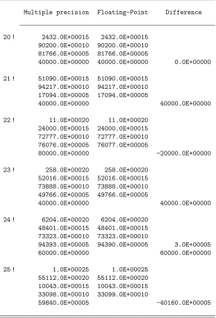
(ii) GNOMBR applied to computation of factorial function
Table : Lost of accuracy with factorial function
Multiple precision Floating-Point Difference
20 ! 2432.0E+00015 2432.0E+00015
90200.0E+00010 90200.0E+00010
81766.0E+00005 81766.0E+00005
40000.0E+00000 40000.0E+00000 0.0E+00000
21 ! 51090.0E+00015 51090.0E+00015
94217.0E+00010 94217.0E+00010
17094.0E+00005 17094.0E+00005
40000.0E+00000 40000.0E+00000
22 ! 11.0E+00020 11.0E+00020
24000.0E+00015 24000.0E+00015
72777.0E+00010 72777.0E+00010
76076.0E+00005 76077.0E+00005
80000.0E+00000 -20000.0E+00000
23 ! 258.0E+00020 258.0E+00020
52016.0E+00015 52016.0E+00015
73888.0E+00010 73888.0E+00010
49766.0E+00005 49766.0E+00005
40000.0E+00000 40000.0E+00000
24 ! 6204.0E+00020 6204.0E+00020
48401.0E+00015 48401.0E+00015
73323.0E+00010 73323.0E+00010
94393.0E+00005 94390.0E+00005 3.0E+00005
60000.0E+00000 60000.0E+00000
25 ! 1.0E+00025 1.0E+00025
55112.0E+00020 55112.0E+00020
10043.0E+00015 10043.0E+00015
33098.0E+00010 33099.0E+00010
3. - Conclusion
In our paper, we have recalled the accuracy problem, summary presented the main solutions available, and an application of our own multiple precision arithmetic tool to an input-output model. Such tools are promising although confidential. Indeed, the capabilities of computers are increasing so that, we can assert that we could still increase accuracy of scientific computations31.
However, we have to specify that even if we could obtain a very high accuracy of the computation, it doesn’t necessarily mean that we would have increased the number or significative digits in the results. If the significant digit’s size of an observation is low, e.g. : 4 digits, even if we obtain a result with 20 digits, only 4 digits are significant32. We have only bounded the
dif-fusion of floating-point round’s error. Also, the main use of such arithmetics for macroeconomic or econometric models, is to decrease floating point error diffusion.
Nevertheless, we believe that two economic applications could use such tools to increase significant digits. Firstly, in the modelling of the Chaos Theory we could use such tools to determine the stability of systems ac-cording to the initial conditions33. Secondly, we believe that we could use
multiple precision arithmetics to make counting process (e.g. : Ap
n = (nn−!p)!
and Cp
n = p!(nn−!p)!) to evaluate precisely the number of individuals in an
Agent-Based computational or Artificial life large simulation.
31. - The only constraint is the size of the needed memory and the computation duration - see V.Ménissier,Arithmétique exacte : conception, algorithmique et performances d’une implantation informatique en précision arbitraire, Thèse de Doctorat, Université de Paris VI, 1994.
32. - About the general problem of error’s measurement see J.Taylor (1996). About the economic observation and account, see O.Morgenstern (1950). As measurement, a datum has got an uncertainty part : the last digits. Jerrell M.E. (op.cit., 1997) has used arithmetic interval to decrease the effect of uncertainty on input-output models.
33. - About an overview of chaotic dynamics, see G.Abraham-Frois & E.Berrebi ( In-stabilité, cycles, chaos,Paris, Economica, 1995, pp.207-61). The authors explain that the logistic function used in the Day’s Model (R.H.Day, "Irregular Growth Cycles",American Economic Review, 72, 1982, pp.406-14.), such as the following : un+1 = a.un.(1−un),
with a = 3.6 provides very different results because of the floating point round’s error. Indeed, if we initiate the series withua
1 = 0.2 andub1 = 0.2000001, after 10000 iterations
the difference betweenua
1andub1was more than 50 %. We have usedGNOMBR to implement
These two ways could be taken, if we agree to increase accuracy memory size and duration computation34. But despite the advantage of technical
progress, we still have to round some results, for example, when result is a number with an infinite digit’s size (rational number, or from combination with e orπ).
4. - References
Alefeld G. & J.Herzberger, Introduction to Interval Computations, New York, Academic Press, 1983.
Avizienis A., "Signed Digit Number Representations for Fast Parallel Arithmetic",IRE Transactions on Electronic Computers, N˚10, 1961, pp.389-400.
Berstel J., J.E.Pin & M.Pocchiola,Mathématiques et informatique - tome 2 Combinatoire et arithmétique, Paris, Ediscience international, Informa-tique, 1991, 257 p. + Programmes.
Buda R., "Présentation d’un outil de contrôle de la précision des calculs en modélisation macro-économétrique",Document de travail GAMA, Université de Paris X-Nanterre, août, 1996, 21 p. + Le logicielGNOMBR.
——–, "SIMUL - Manuel de références et guide d’utilisation version 3.1",
Document de travail GAMA, Université de Paris X-Nanterre, 1999, 60 p. + Le logiciel SIMUL.
——–, "Les algorithmes de la modélisation - une présentation critique pour la modélisation économique",Document de travail ModemN˚01-44, Uni-versité de Paris X-Nanterre, juil., 2001, 97 p.
Daumas M. & J.M.Muller (Eds),Qualité des calculs sur ordinateur - vers des arithmétiques plus fiables ?, Paris, Masson, Informatique, 1997, 164 p.
Dumontet J., Vignes J., "Algorithme de dérivation numérique", RAIRO, Vol.1, 1989.
Jerrell M.E., "Interval Arithmetic for Input-Output Models with Inexact Data", Computational Economics, 1997, 10(1), pp.89-100.
Knuth D.E., The Art of Programming - tome 2, Seminumerical Algo-rithms, (Third ed.), Reading (Mass.), Addison-Wesley, 1997, 762 p.
Kulisch U., "Advanced Arithmetic for the Digital Computer, Design of Arithmetic Units", Electronic Notes in Theoretical Computer Science, 24 , Apr. 2000.a, 63 p.
——–, "Interval Arithmetic in Forte Fortran",Technical White Paper Sun Microsystems, Palo Alto, 2000.b, 54 p.
34. - This size of our Turbo-Pascal software now depends on the RAM limit of the DOS, but it exist some techniques to remove this limit. Let’s quote M.S.Khanniche & S.H.Yong ("A Solution to Memory Limit of DOS Based Large Finite Element Programs",
Kulisch U., W.M.Miranker,Computer Arithmetic in Theory and Practice, New York, Academic Press, 1981.
La Porte M., Vignes J., Algorithmiques numériques - Tome 1, Paris, Tech-niq, 1974, 226 p.
Maillé M., "Some Methods to Estimate Accuracy of Measurements or Nu-merical Computations", Processing of Mathematics for Computer, Congress AFCET, 1982.
Morgenstern O., On the Accuracy of Economic Observations, Princeton, Princeton University Press, 1950.
Moore R.E., Interval Analysis, Prentice-Hall, Englewood Cliffs (N.J.), 1966.
Muller J.M.,Arithmétiques des ordinateurs - opérateurs et fonctions élé-mentaires, Paris, Masson, Études et recherches en informatique, 1989, 214 p.
Pichat M. & J.Vignes, Ingéniérie du contrôle de la précision des calculs sur ordinateurs, Paris, Technip, Informatique, 1993, 233 p. + Programmes.
Sofronioua M. & G.Spaletta, "Precise numerical computation", Journal of Logic and Algebraic Programming, 64(1), Jul., 2005, pp.113-134.
Taylor J.,An Introduction to Error Analysis - : The Study of Uncertain-ties in Physical Measurements, Enfield (New Hampshire), University Science Books, 1996, 327 p.