Volume 44– No.21, April 2012
Analysis of Facial Expression using LBP and Artificial
Neural Network
Renuka R. Londhe
College of Computer Science and IT, Latur Affiliated to S.R.T.M. University, Nanded
Maharashtra, INDIA.
Vrushsen P. Pawar
Associate Professor, S.R.T.M. University, Nanded,
Maharashtra, INDIA
ABSTRACT
Facial Expression Recognition is rapidly becoming area of interest in computer science and human computer interaction. The most expressive way of displaying the emotions by human is through the facial expressions. Local Binary Patterns are widely used for texture classification. In this research paper, we have projected a method for facial expression recognition using Local Binary Patterns (LBP) as features and Artificial Neural Network as a classification tool and we developed associated scheme. The six universal expressions i.e. anger, Generalized Feed-forward Neural Network recognizes disgust, fear, happy, sad, and surprise as well as seventh one neutral. The Neural Network trained and tested by using Levenberg - Marquart (LM) nonlinear optimization algorithm. We are able to attain 93.3 % classification rate with testing performance 0.0573.
Keywords
Facial Expressions, Human Computer Interaction, Local Binary Patterns, Artificial Neural Network.
1.
INTRODUCTION
The computer-based recognition of facial expression has received a lot of attention in recent years because the analysis of facial expression or behavior would be beneficial for different fields such as lawyers, the police, and security agents, who are interested in issues concerning dishonesty and attitude. The eventual goal in research area is the realization of intelligent and transparent communication between human being and machines. Some researchers used only four expressions for analysis using computer and some used six expressions. We have used JAFFE database with seven expressions for analysis through the computer. Several facial expression recognition methods proposed in literature are for example Facial Action Coding System (FACS) [1] [2] Facial Point Tracking [3] and Moment Invariant. Ekman and Friesen [1] developed the Facial Action Coding System (FACS) for describing expressions, such as anger, disgust, fear, happy, neutral, sad, and surprise. The Maja Pantic [4] did machine analysis of facial expressions. James J. Lien and Takeo Kanade have developed Automatic facial expression recognition system based on FACS Action Units in 1998 [5]. They have used affine transformation for image normalization and facial feature point tracking method for feature extraction as well as Hidden Marko Model (HMM) used for
classification. L. Ma. and K. Khorasani developed Constructive Feed-forward Neural Network for facial expression recognition [6]. They generated the difference image from Neutral and expression image, 2-D DCT coefficients of difference images considered as input to the constructive neural network. Praseeda Lekshmi. V and Dr. M. Sasikumar proposed a Neural Network Based Facial Expression Analysis using Gabor Wavelets. They used Gabor Wavelets as a feature extraction method and neural network as a classification technique [7]. T. Ojala first introduced basic Local Binary Pattern operator in 1996. For texture, classification LBP was developed [8]. Timo Ojala and Topi Maenppaa proposed an approach for Multi-resolution gray scale and rotation invariant texture classification with Local Binary Patterns. This approach was very robust in terms of gray scale variations. Computational simplicity is the advantage of LBP. LBP operator can realize a few operations in a small neighborhood. Therefore, LBP operators and its extended versions used for different applications like face recognition, describing the region of interest, object recognition, fingerprint verification and facial expression recognition. Due to the computational simplicity, robustness and accuracy in results, we have decided to use the LBP operator for feature extraction and artificial neural network for classification. This paper organized as follows. Section 2 introduces feature extraction technique i.e. Local Binary Pattern, facial expression description with LBP and ULBP. Section 3 describes neural network process like architecture of neural network and training algorithm. Section 4 depicts the experimental results with database and it discusses the performance, measures and accuracy levels of classification. Finally, in section 5 conclusions are drawn.
2.
FEATURE EXTRACTION
2.1 Local Binary Patterns
For texture description Local binary patterns (LBP) operator is originally designed [8]. LBP encode the pixel wise information in the texture images. The operator assigns a label to every pixel of an image by thresholding the 3×3-neighborhood of each pixel with the center pixel value and considering the result as a binary number. See Fig. 1 for an illustration of basic LBP operator. LBP code of each pixel in the image computed as follows:
11, 0
, 0, 0
0
(
)2 , ( )
N
i x
N R i c x
i
LBP
s n
n
s x
Fig 1: LBP Operator
Where
c
n
is the gray value of the central pixel,n
i is the gray value ofth
i
neighboring pixel,i
0,…, N-1, N is the total number of involved neighboring pixels and R is the radius of the neighborhood which determines how far neighboring pixels are located away from the center pixel. S(x) = 1 if x ≥ 0 else S(x) = 0. The value of N is assigned according to the value of R is suggested in [8] in our implementation N = 8 when R = 1. Supposethe coordinate of
n
c is (0, 0) then the coordinates ofn
i are( cos(2
R
i N R
/
), sin(2
i N
/
))
.
Interpolation is used to estimate the gray values of neighbors that are not in the image grids. Suppose the image is of size M X N. After applying LBP pattern for each pixel, a histogram is built to represent the texture image:
, 1 1
1, 0,
( )
(
( , ), ),
[0, ],
( , )
M N
N R
i j
x y otherwise
H k
f LBP
i j k k
K
f x y
(2)
Where, K is the maximal LBP pattern value.
Uniform patterns are the extension to original LBP operator. A local binary pattern is called uniform if the binary patterns contain at most two bitwise transitions from 0 to 1 or vice versa when the bit pattern is circular. For example 00000000 (0 transitions), 01110000 (2 transitions) and 11001111 (2 transitions) are uniform where as the patterns 11001001 (4 transitions) and 01010011 (5 transitions) are not uniform. In the computation of LBP histogram, uniform patterns used so that histogram has a separate bin for every pattern and all non-uniform patterns assigned to a single bin. Following
notation used for the LBP operator:
LBP
N Ru,2 The subscript represents using operator in a (N, R) neighborhood. Subscript u2 stands for using only uniform patterns.2.2
Facial Expression Description
In this work, the LBP method presented in the previous section is used for facial expression description. The procedure consists of using the texture descriptor to build three local descriptions of the face and combining them in to a complete description. It is observed that facial features contributing to facial expressions mainly lie in some regions, such as eye area and mouth area and nose area. Facial classification needs information that is more useful. These regions contain such type of information.
[image:2.595.366.474.317.442.2]Therefore, facial images are divided in to three local regions upper, middle and lower respectively. Texture descriptors extracted from each region independently. The descriptors then concatenated to form a global description of the facial expression. See Fig 2 for an example of a facial expression image divided in to three rectangular regions.
Fig 2: Average face divided into three blocks In this research work, we are applied Uniform local binary patterns. The U (uniform) value of an LBP pattern defined as the number of spatial transitions or bitwise changes in that pattern
1
, 0
1
1 )
1
(
) | (
)
(
) |
| (
)
(
|
N c
N R c
N
i c i c
i
U LBP
s n
n
s n
n
s n
n
s n
n
(3)2.3
Feature vectors
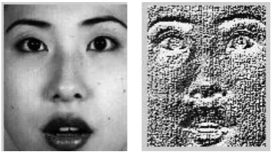
We apply the LBP operator on each pixel of original input image then get the LBP coded image or its histogram shown in Fig. 3c then uniform local binary patterns are collected from the each block of LBP coded images and its histogram is shown in the Fig. 3d.
[image:2.595.321.518.637.750.2]Volume 44– No.21, April 2012
Fig 3: c) Histogram of LBP coded Image
Fig 3: d) Sample Histogram of ULBP (Feature Vector)
Only 59 bins used to represent or show the ULBP histogram of each block. Occurred 59 values of each block used as a feature vector. After combining features of three blocks, we get the feature vector of size 1 X 177 for average image. We are used 210 images from the database; input matrix for classifier is of size 177 X 210.
This methodology divided into following steps:
1. Extract average face from the original images of database;
2. Divide average image in to three blocks such as upper (eyes), middle (nose) and lower (mouth) respectively;
3. Compute the LBP code for each pixel in a block using equation (1);
4. Compute the histogram over the block, using equation (2) of the frequency of each "number" occurring (i.e., each combination of which pixels are smaller and which are greater than the center); 5. Optionally normalize the histogram;
6. Concatenate normalized histograms of all blocks. This gives the feature vector for the average face; and
7. Use artificial neural network (see section 4) to classify these features into different classes such as anger, disgust, fear, happy, neutral, sad and surprise.
3.
ARTIFICIAL NEURAL
NETWORK
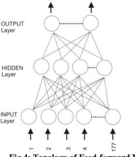
A two layer feed forward neural network with sigmoid activation function is constructed with ten hidden neurons and seven output neurons for classification purpose. Following Fig. 4 depicts topology of neural network. The network training instructed with Levenberg - Marquart (LM) nonlinear optimization algorithm [10]. It is the fastest back propagation algorithm with a combination of steepest descent and the Gauss Newton Method.
Fig 4: Topology of Feed-forward Neural Network
When the current solution is far from the correct one, the algorithm behaves like a steepest descent method: slow, but guaranteed to converge. When the current solution is close to the correct solution, it becomes Gauss-Newton method. Thus, it continuously switches its approach and can make very rapid progress. For iteration in the learning process, the weight vector w is updated as follows
1
k k k
W
w
d
(4)
1[
]
k
T T
d
J
J
I
J
(5)
Where
d
k is search direction,
is damping parameter ofk
th iteration,
is a vector of network errors and J is the Jacobian matrix that contains first derivatives of the network errors with respect to the weights. When the scalar
is zero, this is just Newton’s method, using the approximate Hessian matrix. When
is large, this becomes gradient descent with a small step size. Newton’s method is faster and more accurate near an error minimum, so the aim is to shift towards Newton’s method as quickly as possible. Thus,
decreased after each successful step and increased only when a tentative step would increase the performance function.Out of 210 images, 132 images presented to the network during training, so that the network adjusted according to its error. 32 images are used to measure the network generalization and to halt the network when generalization stops improving. Remaining 32 images are used to perform testing of an independent measure of network performance during and after training. The training stops when a classifier gives a higher accuracy value with minimum training and testing errors.
4.
EXPERIMENTAL RESULTS
[image:3.595.315.455.70.232.2] [image:3.595.81.270.85.289.2]As mentioned in subsection 3, the important features of expressions reflected through the eyes and mouth. Therefore, we extract average face of size 125 x 106 from original image. Again, the average images divided in to three blocks to extract the more features such as upper, middle and lower as shown in Fig 2.
4.1 Performance
The LM training algorithm outperformed in this experiment by classifying the input data in 16 epochs with the average training time of 20 seconds.
[image:4.595.71.284.63.178.2]The performance measured and outcome of the network are as follows
Table 1 Performance Measures
Number of Epochs 16
Training Performance 0.0012 Testing Performance 0.0573 Validation Performance 0.0501 Classification Rate 93.3% Mean Squared Error 1.97453e-2
Percent Error 6.6666e-0
The error measures like Mean Squared Error (MSE) and Percent Error (PE) are recorded. MSE is the mean of the squared error between the desired output and the actual output of the neural network. Fig. 6 depicts performance graph.
Fig 6: Performance Graph
ij
d
processing element j.
Percent Error indicates the fraction of samples, which are misclassified. A value
0
means no misclassifications.0 0
|
|
100
%
P N
ij ij
j i ij
dy
dd
error
NP
dd
(7)Where
P = number of output processing elements N = number of patterns in the training data set
ij
dy
= demoralized network emissions output for pattern i at processing element jij
[image:4.595.313.526.181.547.2]dd
= demoralized desired network emissions output for exemplar i at processing element j.Fig 7: Error Histogram
4.2 Confusion Matrix
[image:4.595.86.268.348.431.2] [image:4.595.316.525.399.559.2] [image:4.595.72.271.502.651.2]Volume 44– No.21, April 2012
Fig 8: Confusion Matrix I
[image:5.595.330.507.72.249.2]As an input, we gave 30 images for each class. Resultant Confusion matrix II illustrates that, 29 images are fall in anger class and remaining one image fall in class 5 i.e. neutral, same misclassification is done with all classes excluding happy class. Therefore, average accuracy of classification is 93.3% misclassification or error rate is 6.7%.
Fig 9: Confusion Matrix II
4.3 Receiver Operator Characteristic
(ROC)
Classification accuracy mostly measured by Receiver Operator Characteristic (ROC) curve, which shows the relationship between false positives and true positives. For each threshold, two values are calculated, the True Positive Ratio (the number of outputs greater or equal to the threshold, divided by the number of one targets), and the False Positive Ratio (the number of outputs less than the threshold, divided by the number of zero targets). The following figure plots the receiver-operating characteristic for each output class. The more each curve cuddles the left and top edges of the plot, the better the classification.
Fig 10: Obtained Receiver Operator Characteristics
5.
CONCLUSION
In this paper, an efficient facial expression representation and classification methodology is proposed. Facial Expression representation based on LBP and Extended LBP called Uniform Local Binary Patterns (ULBP). Feature vectors are computed from histograms of ULBP. These features are classified using the two layer feed forward neural network. For training this network Levenberg - Marquart (LM), nonlinear optimization algorithm is used. The six universal expressions i.e. anger, disgust, fear, happy, sad, and surprise as well as seventh one neutral, are recognized with 100% accuracy for one subject’s images and as high as 93.3% accuracy with the combination of 10 subject’s images.
6.
REFERENCES
[1] Paul Ekman, “Basic Emotions”, University of California, Francisco, USA.
[2] Ioanna-Ourania and George A. Tsihrintzis, “An improved Neural Network based Face Detection and Facial Expression classification system,” IEEE international conference on Systems Man and Cybernetics 2004.
[3] Ying-li Tian, Takeo Kanade, and Jaffery F. Cohn, “Recognizing Action Units for Facial Expression Analysis,” IEEE transaction on PAMI, Vol. 23 No. 2 Feb. 2001.
[4] Maja Pantic and L.L.M. Rothkrantz, “Automatic analysis of facial expressions: The state of the art,” IEEE Trans. PAMI Vol. 22 no. 12 2000.
[5] James J. Lien and Takeo Kanade, “Automated Facial Expression Recognition Based on FACS Action Units”, IEEE published in Proceeding of FG 98 in Nara Japan.
[6] Ma and K. Khorasani, “Facial Expression Recognition Using Constructive Feed forward Neural Networks,” IEEE TRANSACTION ON SYSTEM, MAN AND CYBERNETICS, VOL. 34 NO. 3 JUNE 2004.
[7] Praseeda Lekshmi. V Dr. M. Sasikumar, “A Neural Network Based Facial Expression Analysis using Gabor Wavelets,” Word Academy of Science, Engineering and Technology.