Conspicuous Consumption and Overlapping Generations

Munich Personal RePEc Archive

Conspicuous Consumption and

Overlapping Generations

Wendner, Ronald

Graz University, Austria

2 June 2009

Online at

https://mpra.ub.uni-muenchen.de/15527/

Conspicuous Consumption and Overlapping

Generations

⋆

Ronald Wendner

Department of Economics, University of Graz, Austria Universitaetsstrasse 15, RESOWI-F4,

A-8010 Graz, Austria

E-mail ronald.wendner@uni–graz.at

Web http://www.uni-graz.at/ronald.wendner

Phone +43 316 380 3458

June 2, 2009

Abstract. This paper investigates household decisions, and optimal taxation in an overlapping generations model in which individual utility depends on a weighted av-erage of consumption of ones peers — a “keeping up with the Joneses” consumption externality. In contrast to representative agent economies, the consumption exter-nality generally affects steady state savings and growth rates. The nature of the externality’s impact, however, critically depends on the rate at which labor produc-tivity declines with age. For a (strongly enough) declining labor producproduc-tivity (or when people gradually retire), the consumption externality lowers the steady state propensity to consume out of total wealth. The opposite holds for a constant labor productivity. The market economy can be decentralized by a (reverse) unfunded so-cial security system if the rate of labor productivity decline is high (low). In contrast to previous results, theoptimal steady state capital income tax is zero, in spite of the consumption externality.

Keywords and Phrases: Consumption externality, labor productivity, gradual re-tirement, overlapping generations, keeping up with the Joneses, optimal taxation, capital taxation.

JEL Classification Numbers: D91, E21, O40

⋆_{I thank Carl-Johan Dalgaard, Bill Dupor, Karl Farmer, Robert Hill, Johan Lagerloef, Lorenzo}

1

Introduction

Psychologists have often pointed to the fact that individuals experience happiness by

doing wellrelative to some reference group. In economic terms, this observation refers

to what is calledconspicuous consumption or the desire to keep up with the Joneses.1

The effects of which for household behavior in a market economy and for distortions

are considered in this paper.

Economists have frequently argued that conspicuous consumption is one source for

the low savings rates observed in developed countries. As everyone aims at keeping

up with the Joneses, there is “overconsumption,” and the savings rate is lower than

optimal. But is this a valid argument? This paper will conclude that, in general, this

is not a valid argument.

The phenomenon of conspicuous consumption is not a new one. In the past, many

classical economists assumed that conspicuous consumption or the quest for status

— a consumption externality, in modern terms — is an important component of the

pursuit of self-interest (Kern, 2001). InThe Theory of Moral Sentiments, Adam Smith

notes:

Though it is in order to supply the necessities and conveniences of the

body that the advantages of external fortune are originally recommended

to us, yet we cannot live long in the world without perceiving that the

respect of our equals, our credit and rank in the society we live in, depend

very much upon the degree in which we possess, or are supposed to possess

those advantages. The desire of becoming the proper objects of this respect

... is perhaps the strongest of all our desires (Smith 1759, pp. 348–349).

More recently, the previous literature offers strong evidence of the existence of

con-spicuous consumption. Important contributions include Brekke and Howarth (2002),

Frank (1985, 1999), Johansson-Stenman et al. (2002, 2006), Luttmer (2005), and

Sol-nick and Hemenway (1998, 2005). The existence of externalities has been successful in

1_{In the following, we use the termsconspicuous consumption and (keeping up with the Joneses)}

explaining a number of stylized facts. For example, externalities shed important light

on the implications of status effects for happiness (Easterlin 1995, Frank 1985, Frank

1999, Scitovsky 1992), asset pricing (Abel 1999, Campbell and Cochrane 1999, Dupor

and Liu 2003), optimal tax policy over the business cycle (Ljungqvist and Uhlig 2000),

and optimal redistributive taxation (Boskin and Sheshinski 1978).

This evidence motivates the analysis of the theoretical effects of conspicuous

con-sumption on concon-sumption and savings decisions. As the framework for analysis, we

employ a continuous time overlapping generations (OLG) model, in which individual

labor productivity decreases with age. The representative agent model emerges as a

special case of the employed framework.

This paper offers three main contributions with respect to the prior literature

re-lated to conspicuous consumption. First, conspicuous consumption generally changes

the steady state propensity to consume, consumption (growth) and capital

accumula-tion. The nature of the effects, however, critically depends on the rate at which labor

productivity declines with age. If the rate of decline of the labor productivity is small,

conspicuous consumption raises the steady state propensity to consume, and it lowers

the steady state consumption and capital levels. The opposite is true when the rate of

decline of the labor productivity is high. This result differs from what was shown for

representative agent economies. Rauscher (1997), Brekke and Howarth (2002), Liu

and Turnovsky (2005), and Turnovsky and Monteiro (2007) demonstrate that in a

representative agent economy with exogenous labor supply, a consumption

external-ity has no impact on the steady state equilibrium. In their settings, the steady state

capital stock is fully determined by the Keynes-Ramsey rule, independently of a

con-sumption externality. In this paper, we show that a concon-sumption externality always

has effects on the steady state equilibrium in an overlapping generations framework.

This has been observed already by Garriga (2006), Wendner (2007) and Fisher et

al. (2009). What has not been observed, however, is the fact that conspicuous

con-sumption may either rise or lower the propensity to consume, depending on the rate

individual consumption levels change with age. As a consequence of the continuous

inflow of new generations, individual and average consumption levels generally differ

from each other. This opens a channel for the externality to have an impact on

con-sumption and capital, as the steady state capital stock is not determined anymore

by the Keynes-Ramsey rule. The rate at which labor productivity declines with age

affects the differences between individual and average consumption growth rates, and

thereby, the effects of conspicuous consumption.

Second, the socially optimal allocation can be decentralized by a tax on capital

income and an unfunded social security system. In contrast to the results of Abel

(2005) and Garriga (2006), however, the optimal steady state capital income tax rate

equals zero, in spite of the presence of a consumption externality. The difference in

results is caused by the fact that the propensity to consume is age-dependent in the

two-period OLG model, while it is independent of age in the continuous time OLG

model. Implementation of an optimal social security system affects a household’s

propensity to consume — thereby the intergenerational consumption growth rate —

in the two-period OLG model. This effect, which is corrected for by a tax on capital

income, is not seen in the continuous time OLG model.

Third, conspicuous consumption always introduces a distortion in the continuous

time OLG model. If the rate at which labor productivity declines is high (low) an

unfunded social security system (a reverse unfunded social security system) is capable

of decentralizing the optimal allocation. With a high (low) rate of labor productivity

decline, conspicuous consumption causes steady state overconsumption

(undercon-sumption) which requires the optimal transfer scheme to increase (decrease) with age.

The results emphasize the significance of the rate at which labor productivity

declines with age for the effects of conspicuous consumption. One direct implication

of the above results is the following. Conspicuous consumption either raises the

propensity to consume (in case of a low rate of labor productivity decline), or it

yields overconsumption (in case of a high rate of labor productivity decline). But it

Section 2 of the paper presents the economy’s structure. Section 3 considers the

steady state effects of conspicuous consumption in a market economy. Section 4 sets

up a command optimum and shows that the optimal allocation can be decentralized

by a (reverse) unfunded social security system. It discusses the impact of conspicuous

consumption on the optimal social security system. Section 5 concludes the paper.

The appendix contains a number of derivations and proofs that were distracting when

placed in the main text.

2

The Economy’s Structure

In this section, we augment the standard continuous time overlapping generations

model by a “keeping up with the Joneses” consumption externality (conspicuous

con-sumption). Individual utility not only depends on own consumption but also on a

weighted average of consumption by others.

Population. An individual born at time v (“vintage”) is uncertain about the length

of his or her life. As in Blanchard (1985) and Buiter (1988), both the instantaneous

probability of death of a cohort (the death or mortality rate), d, and the birth rate,

b, are age-independent and constant over time.

At time t, the population size is L(t). At each instant of time, a new cohort is

born, the size of which is b L(t). Also, at timet, the mass of people who die is d L(t).

Accordingly, for a large population size, the rate of population growth is

n =b−d . (1)

Population at some date t1 is given by: L(t1) = L(t0)en(t1−t0). Without loss of

generality, L(0) = 1. Consequently,L(t) =en t_.

Denote the size of a vintage-v cohort at time t by L(v, t). Under this

popula-tion structure L(v, t) = L(v, v)e−d(t−v) _{= b L(v)e}−d(t−v) _{= b e}n v_e−d(t−v) _{= b e}b v−d t_.

Similarly, the share of a vintage-v cohort in total population at timet is:

The expected remaining lifetime of any agent is: d−1_.2 _{In the following, we focus on}

the case without population growth:

n= 0, L(t) = 1. (3)

As we conceptually distinguish the birth rate from the death rate, we will clarify

which of the results are driven by the perpetual inflow of cohorts (b >0) and which

are driven by the finiteness of lifetime (d >0).

Households. Time-tutility of a vintage-v household is a functionu(.) of consumption

c(v, t). The first argument in c(.) refers to the birth date, and the second argument

refers to time. At time t, an individual household not only cares about its own

consumption, but also about how own consumption compares to some consumption

reference level, x(v, t), which is discussed below. Instantaneous utility is then given

by u(c(v, t), x(v, t)).

In this paper, we consider the standard case of a CRRA utility function. We follow

Dupor and Liu (2003) in specifying the felicity function3 _as:

u(c(v, t), x(v, t)) =

h

c(v, t)1−1η x(v, t)−

η

1−η

i1−σ

−1

1−σ =

·

c(v, t) ³_xc(₍v,t_v,t)₎´

η

1−η

¸1−σ

−1

1−σ ,

(4)

where 0≤η <1 is called the “reference parameter,” which measures the importance of the consumption reference level. Ifη = 0, utility depends only on own consumption,

and the model reduces to the usual model with interpersonally separable utility. If

the reference parameter is strictly positive,ηintroduces a keeping up with the Joneses

consumption externality (conspicuous consumption). The externality is reflected by

the fact that utility is also derived from own consumption relative to a reference

level (roughly, relative to others). The reference parameter represents the fraction of

marginal utility of consumption stemming from a rise in this fraction, c(v, t)/x(v, t).4

2_{As a special case, the representative-agent model emerges from the perpetual youth model by}

settingb= 0, andd=−n.

3_{This case is often referred to as the “multiplicative specification” (Gal´ı, 1994).}

4_{Johansson-Stenman et al. (2002) call this fraction the “marginal degree of positionality.”}

If, say, η = 0.2, then 20% of marginal utility of consumption stems from a rise in

c(v, t)/x(v, t), while the remaining 80% directly come from a rise in own consumption

c(v, t), holding constant the fraction c(v, t)/x(v, t).

Parameter σ governs the intertemporal elasticity of substitution. If η = 0, the

intertemporal elasticity of substitution is given by σ−1_{. If, however, η >0, all}

param-eters, σ,η, andεdetermine the elasticity of substitution between consumption at any

two points in time.

Consumption Reference Level. The consumption reference level of a household is

a weighted geometric mean of others’ consumptions of its own cohort, ¯c(v, t), and

average consumption of society, c(t):

x(v, t) = ¯c(v, t)εc(t)1−ε, 0≤ε <1, (5)

whereεand (1−ε) represent the weights attached to consumption of one’s own cohort and average consumption of society, c(t) ≡ Rt

−∞ l(v, t)c(v, t)dv respectively. In the

special case in which ε approaches unity (in which ε = 0) consumption of one’s own

cohort (of society) represents the only frame of reference for consumption.

Sign Restrictions. First, 0≤η <1 ensures positive marginal utility of consumption and quasiconcavity of the utility function. Second, σ > 1, which is overwhelmingly

suggested by the literature, ensures decreasing marginal utility and strict concavity

of u(.)|¯c(v,t)=c(v,t) in c(v, t). In particular, these sign restrictions imply:

˜

σ≡ (σ−η)−ε η(σ−1)

1−η ≥σ >1. (6)

At time t, expected remaining lifetime utility of a cohort born at date v is:

U(v, t) =

Z ∞

t

u(c(v, s), x(v, s))e−(ρ+d) (s−t)ds , (7)

where ρ is the household’s pure rate of time preference. The possibility of death

(d > 0) leads to a subjective discount rate (ρ+d) higher than the pure rate of time

Production. There is a large number of competitive, identical firms. The

representa-tive firm produces a homogeneous output, Y, according to

Y(t) =A K(t)α_N(t)1−α_{, A >0, 0< α <1, (8)}

where K and N are capital and effective labor services, and A is total factor

pro-ductivity. Any individual laborer’s productivity depends on her age. In particular,

age-dependent productivity, π(t−v), develops according to

π(t−v) =e−λ(t−v), λ(˜σ−1)< ρ+d , (9)

where we refer toλas the rate at which individual labor productivity declines with age

— although one might also think of λ as the rate of (exogenous) gradual retirement.

The formulation can be extended to accommodate more complex paths of productivity

profiles (e.g., an inverse U-shaped pattern). In the following, however, the main

purpose of considering nonconstant productivity paths is to make the present value of

future wage payments dependent on the profile of individual labor productivity. The

simplest formulation of which is given by (9).

Labor supply, L(t), and effective labor supply,N(t), are related as follows:

N(t) =

Z t

−∞

π(t−v)L(v, t)dv=L(t)

Z t

−∞

b e−(b+λ)(t−v)dv =L(t) b

b+λ, (10)

that is, aggregate effective labor supply declines in λ. Let y(t) ≡ Y(t)/L(t), and

k(t)≡K(t)/L(t) denote the average product and the capital labor ratio respectively:

y(t) = A k(t)α

·

b b+λ

¸1−α

. (11)

Firms maximize profits and hire factors from households on competitive factor

markets:

r(t) +δ=α A k(t)(α−1)

·

b b+λ

¸1−α

, (12)

w(v, t) = (1−α)A k(t)α

·

b b+λ

¸−α

e−λ(t−v), (13)

w(t) =

Z t

−∞

l(v, t)w(v, t)dv = (1−α)A k(t)α

·

b b+λ

¸1−α

where r(t) is the rate of interest, w(v, t) is the wage rate, w(t) is the wage rate per

effective unit of labor, and δ is the rate of depreciation of capital. According to the

resource constraint, the average stock of capital evolves according to:

˙

k(t) = y(t)−c(t)−δ k(t), (15)

where y(t) is negatively affected by the productivity parameter λ, as seen in (11).

Consumption. Households do not have a bequest motive. They can buy fair life

annuity contracts from life insurance companies, for which they pay or receive the

annuity rate of interestrA_{(t). The contracts are canceled upon death of an individual.}

Actuarial fairness requires rA_{(t) = r(t) +d. The annuity interest factor is given by:}

RA_(t

0, t1)≡

Rt1

t0 [r(s) +d]d s.

Every household inelastically supplies labor services and chooses consumption at

allt≥v such as to maximize expected lifetime utility (7) subject to its intertemporal budget constraint:5

a(v, t) +h(v, t)−

Z ∞

t

c(v, s)e−RA(t,s)ds= 0, (16)

where a(v, t) stands for time-t assets (accumulated wealth) of a vintage-v household,

and human wealthh(v, t)≡R∞

t w(v, s)e−R

A_(t,s)

dsis the discounted integral of present

and future wage payments. In the market framework, a household does not consider

the impact of its individual consumption on the consumption reference level.

Individual consumption levels are derived by applying Pontryagin’s maximum

prin-ciple, in the appendix. Define:

∆(t)≡

Z ∞

t e

Rs t

r(τ)−ρ ˜

σ +

˜

σ−σ ˜

σ

˙

c(τ)

c(τ)d τ−R

A_(t,s)

d s . (17)

Then:

c(v, t) = ∆−1[a(v, t) +h(v, t)], c(t, t) = ∆−1h(t, t), (18)

5 _{The transversality condition required to prevent households from running Ponzi schemes is:}

lims→∞e −RA(t,s)

a(v, s) = 0, or, equivalently, lims→∞ µa(s)e −(ρ+d)s

a(v, s) = 0, where µa is the

where the second expression follows from the fact that there is no operative bequest

motive: a(t, t) = 0. Consumption levels are proportional to (accumulated and human)

wealth, with the age-independent factor of proportionality given by: ∆−1_{(t), which}

can be interpreted as the propensity to consume out of total wealth. Notice that at

any given point in time, consumption levels are not equal across cohorts.

Individual consumption growth rates are given by:

gc(v,t) ≡

˙

c(v, t)

c(v, t) =

[r(t)−ρ] ˜

σ +

˜

σ−σ

˜

σ

˙

c(t)

c(t). (19)

Consumption growth rates are equal across cohorts. Individual consumption growth

rates do not only depend on the rate of interest and the pure rate of time preference,

but they also depend positively on the growth rate of average consumption.

Average accumulated wealth,a(t), is given bya(t)≡Rt

−∞ l(v, t)a(v, t)dv. Capital

market clearing requires:

a(t) =k(t). (20)

Finally, average human wealth, h(t), is:

h(t) =

Z t

−∞

l(v, t)h(v, t)dv= b

b+λh(t, t) = b b+λ

Z ∞

t

w(s)e−RA(t,s)e−λ(s−t)d s .

(21)

We are now ready to represent a perfect foresight equilibrium by a series of three

differential equations in the variables c, k, ∆:

˙

c(t)

c(t) =

r(t)−ρ

σ +

˜

σ σ

·

λ−(b+λ) ∆−1 k(t)

c(t)

¸

(M.1)

˙

k(t) =A k(t)α

·

b b+λ

¸1−α

−c(t)−δ k(t), (M.2)

˙

∆(t) =−1 + ∆(t)

·

r(t) +d−r(t)−ρ

˜

σ −

˜

σ−σ

˜

σ

˙

c(t)

c(t)

¸

, (M.3)

where r(t) = α A k(t)(α−1) £ _b

b+λ

¤1−α

−δ. Equation (M.1) is derived by differentiation of average consumption with respect to time and using (19).6 _{Equation (M.2) restates}

the resource constraint. Equation (M.3) follows right from differentiation of (17).

6_{Denote individual consumption growth by g}

c(v,t). Here, we consider the fact ˙c(t) = b c(t, t)−

b c(t) +gc(v,t)c(t), where [b c(t, t)−b c(t)] = b∆−1h(t, t)−b c(t) = b∆−1(b+λ)/b h(t)−b c(t).

Considering both ∆−1_{h(t) = [c(t)−∆}−1_{k(t)] and ∆}−1_{(t) =c(t)/[k(t)+h(t)], yields: b c(t, t)−b c(t) =}

If b = λ = d = 0, the standard Ramsey model emerges. In a steady state – if

˙

c = 0 – equation (M.1) represents the Keynes-Ramsey rule: r(k) = ρ. If, however,

(b, λ) ≫ 0, there is a continuous inflow of new cohorts without accumulated wealth (b >0), and there is a continuous decay of human wealth of any existing cohort over

time (λ >0). As a consequence, the wealth (human and accumulated) of a new cohort

may differ from the average wealth, which gives rise to the generation replacement

effect.

Generation Replacement Effect. A household’s individual consumption growth rate is

independent of age. The generation replacement effect (GRE) refers to the difference

between average and individual consumption growth rates, which is based on the fact

that individual consumption levels change with age: c(v, t) 6= c(t). Analytically, the GRE — captured by the term Γ(t) — is determined by:

Definition 1 Γ(t)≡λ−(b+λ)_k(tk₎₊(t_h)_(t) =λ−(b+λ) ∆−1_(t)k(t)

c(t).

Employing Definition 1,

gc(t)≡

˙

c(t)

c(t) =gc(v,t)(t) + Γ(t). (22)

In particular,gc(t)Rgc(v,t)(t)⇔Γ(t)R0. If Γ(t)6= 0, there exists a GRE. The GRE

is not present in the Ramsey model, where b= 0.

Lemma 1 (Generation Replacement Effect)

(i) {h(t, t) = [a(t) +h(t)]} ∨ {b= 0} ⇔ Γ(t) = 0. (ii) (b > 0)∧(λ= 0) ⇒ Γ(t)<0⇔gc(t)< gc(v,t).

(iii) Suppose b > 0. Then there exists λ˜(t) > 0, such that Γ(t) = 0, where λ˜(t) =

b k(t)/h(t). Moreover, for λ _≶λ˜(t)⇔Γ(t)_≶0.

Proof. See appendix. ||

In the model of perpetual youth, the average consumption growth rate may differ

from the individual consumption growth rate. With b >0, newborn cohorts without

accumulated wealth is lower than average accumulated wealth: 0 = a(t, t)< a(t). If

λ > 0, however, a newborn cohort’s human wealth is greater than average human

wealth: h(t, t) =h(t) (b+λ)/b > h(t). The rate of labor productivity decline decides

on whether the total (human and accumulated) wealth of a newborn cohort is lower

or greater than average total wealth. If λ < λ˜, h(t, t) < h(t) +a(t), in which case

c(t, t)< c(t). If λ >λ˜,h(t, t)> h(t) +a(t), in which case c(t, t)> c(t).

At the same time, individual consumption growth rates are independent of age and

equal among all cohorts at any given point in time. By the very fact that newborn

cohorts — with consumption levels different from the average consumption levels —

continuously enter the economy, the average consumption growth rate differs from

the individual consumption growth rate. Only in the special case in which h(t, t) =

h(t) +a(t), there is no GRE: Γ(t) = 0, and gc(t) = gc(v,t).

Strict positivity of the instantaneous birth rate (but not of the death rate) is

necessary for the GRE to occur. The GRE occurs even in the setting of a perpetual

youth model with infinitely-lived agents, that is, with b >0, d= 0, as in Weil (1989).

It is the inflow of newborn cohorts whose total wealth is different from the average

wealth, which causes the GRE.

3

The Effects of Externalities

In the following section, we consider the effects of conspicuous consumption on

bal-anced growth paths (steady state equilibria). For steady state values, we omit the

time indexes as of here. In the market economy, a steady state equilibrium is given

by ˙c= ˙k = ˙∆ = 0:

0 = r(k)−ρ

σ +

˜

σ σ

·

λ−(b+λ) ∆−1 k

c

¸

= r(k)−ρ ˜

σ + Γ, (M.SS.1)

c=y(k)−δ k , (M.SS.2)

∆−1 =r(k) +d− r(k)−ρ

˜

σ . (M.SS.3)

From (M.SS.1)–(M.SS.3) it follows that a steady state equilibrium can be represented

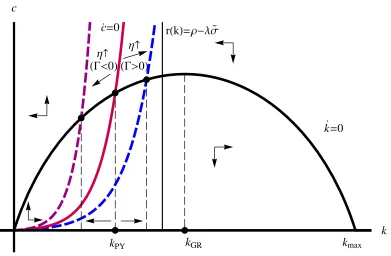
k =0 c =0

Η­

HG<0L

Η­

HG>0L

kGR kmax

rHkL=Ρ-Λӎ

kPY

k c

Figure 1: Impact of the Consumption Externality

Figure 1 displays the ˙k= 0– and ˙c= 0–lines in (k, c) space. The point of intersection

(with k >0, c >0) shows the nontrivial steady state equilibrium.7 _{The properties of}

the ˙k= 0– and ˙c= 0–lines, as displayed in the figure, are discussed in the appendix.

Arrows indicate the movements of trajectories.

Figure 1 also shows an asymptote for the ˙c = 0-line at: r(k) = ρ−λ˜σ. The asymptote implies an important fact. At a steady state equilibrium, r(k)> ρ−λσ˜. Ifλ >0,r(k) is allowed to assume a valuelower thanρin a steady state. In particular,

we note:

Lemma 2 In a steady state equilibrium,

(i) [r(k)−ρ]R0⇔Γ⋚0,

(ii)there exists λ >˜ 0 such that Γ(˜λ) = 0,

where λ˜=b h(1−_αα) _ρ+ρ+_d+δ_λi−1 >0,

(iii) Γ(λ)≷0⇔λ≷λ˜.

Proof. See appendix. ||

Clearly, Γ > 0 does not imply dynamic inefficiency. Noticing that capital increases

in λ, we define ¯λ to be the value of λ, which implies the golden rule capital stock:

r(k(¯λ)) = 0. From above, r(k(˜λ)) = ρ >0. Thus, ¯λ > λ˜. Dynamic efficiency occurs

for all λ ∈[0,λ¯]. If, in addition λ∈[˜λ,λ¯], then Γ>0.8

We can now analyze the impact of externalities on steady state equilibria. Figure

1 indicates that (a rise in the strength of) conspicuous consumption tilts the ˙c =

0-line either anticlockwise or clockwise. The effects of the consumption externality are

ambiguous, depending on the sign of Γ.

Proposition 1 (Effects of the Consumption Externality) Suppose 0 ≤ λ <λ¯. In the market economy, the consumption externality has an ambiguous impact on the

steady state allocation. In particular:

Γ_⋚0⇔ ∂ c

∂ η ⋚0, ∂ k ∂ η ⋚0,

∂(c/k)

∂ η R0.

Proof. See appendix.||

Proposition 1 displays four main insights. First, given Γ 6= 0, a consumption exter-nality — even with exogenous labor supply — does have a steady state impact on

consumption, capital, and the propensity to consume out of accumulated wealth,c/k.

The nature of the impact of a consumption externality, however, depends on the sign

of Γ. If Γ < 0, the consumption externality raises the propensity to consume out of

wealth. If Γ>0, however conspicuous consumption lowers the steady state propensity

to consume out of wealth, as explained below.

This result is in tension with the previous literature (Liu and Turnovsky 2005,

Turnovsky and Monteiro 2007) that shows that consumption externalities, with

ex-ogenous labor supply, do not have an impact on the steady state allocation in

rep-resentative agent models. This seeming contradiction can be rectified, however. The

representative agent model is a special case of the present framework, with b=d= 0.

8_{The transversality conditions require a(v, t) to increase at a rate lower thanr+d, in a steady}

By Lemma 1(i), Γ = 0 in the representative agent model. As a consequence, Lemma

2(i) implies r(k) =ρwhenever Γ = 0, in which case the consumption externality does

not have an impact on the steady state equilibrium indeed.

In the framework of overlapping generation economies, both Wendner (2007) and

Fisher et al. (2009) notice that consumption externalities raise the propensity to

consume out of accumulated wealth, in spite of exogenous labor supply. Both papers,

however, fail to recognize that the effects of conspicuous consumption are ambiguous

and — depending on the rate of labor productivity decline — can go either way.

Second, ifλ <λ˜ then Γ<0, according to Lemma 1(iii). For this case, Proposition

1 shows that the keeping up with the Joneses consumption externality raises the steady

state propensity to consume out of accumulated wealth,c/k. Intuitively, consumption

is a positional good. A household not only derives utility from its own consumption

level but also from the consumption-to-reference level ratio (roughly, from

above-average consumption). The consumption externality provides an incentive to raise

individual consumption relative to the reference level.

Initially, for a given level k, a rise in η raises individual consumption levels and

lowers the individual consumption growth rate. This reaction is seen by restating the

steady state version of Euler equation (19) as follows:

r(k) =ρ+ ˜σ gc(v,.). (23)

For ¯c(v, t) = c(v, t), the term ˜σ represents the (absolute) consumption elasticity of

marginal utility. A rise in η raises the elasticity of marginal utility (˜ση > 0). That

is, for a given positive growth rate of individual consumption, a rise in η induces

the marginal utility to decline too strongly over time (the right hand side of the

Euler equation exceeds the left hand side), and households will aim to smooth their

consumption paths. Consequently, households will bring some future consumption

forward to the present and, according to (23), lower the consumption growth rate.

As, initially, every individual household raises its consumption level, average

con-sumption rises as well. This reaction, in turn, implies a lowering in aggregate savings.

by a lower level of k. Consequently, average consumption declines as well, as shown

in Figure 1. As the production function is strictly concave, the average product of

capital declines in k. That is, ∂(y/k)/(∂ k) = ∂(c/k)/(∂ k) < 0. As k declines, the

steady state propensity to consume out of accumulated wealth, c/k, rises.

Third, Lemma 1(iii) shows that λ > λ˜ implies Γ > 0. In this case, Proposition

1 demonstrates that the keeping up with the Joneses consumption externality lowers

the propensity to consume out of accumulated wealth, and it raises average steady

state consumption and capital levels. At first sight, this result does not square well

with intuition. To gain insight, it is important to note that one’s relative consumption

(c(v, t)/x(v, t)) not only matters today but also in the future. Consuming more today

rises one’s relative consumption, ceteris paribus. This rise comes at a cost, however.

Consuming more today lowers tomorrow’s consumption level, thereby tomorrow’s

rel-ative consumption, ceteris paribus. In contrast, lowering one’s consumption today

allows for a higher level of consumption (and a better relative position, other things

being equal) in the future. If Γ>0, households prefer the latter option.

If Γ > 0, it follows from Lemma 2(i) that r(k) < ρ. In this case, the human

wealth of a newborn generation exceeds the average total wealth. Consequently, the

individual steady state consumption growth rate is negative. That is, an individual’s

consumption level declines over time, and its marginal utility of consumption rises

over time. As above, an increase in η raises the elasticity of marginal utility. As a

consequence, for a given gc(v,.), marginal utility increases at too big a rate over time.

Households will postpone consumption and, according to (23), lower the (negative)

consumption growth rate.

Initially, for given levels of c and k, Euler equation (23) requires the individual

consumption growth rate to increase (gc(v,.) to become less negative) as of a rise in

η. This rise is achieved by initially lowering the individual consumption levels. As,

initially, every individual household lowers its consumption level, average consumption

declines as well. This lowering implies a rise in average savings. Subsequently the

to consume out of accumulated wealth is lower (by strict concavity of the production

function).

Fourth, Proposition 1 also shows a special case: b >0 and Γ = 0. In this

“knife-edge” case, the optimal individual consumption growth rate is zero. While a rise in

η still raises the elasticity of marginal utility, it implies no change on gc(v,.).

Conse-quently, there is neither an initial nor a steady state response to the change in η. In

this case, the consumption externality does not have an impact on the steady state

equilibrium. It is important to note, however, that this special case can only occur if

λ= ˜λ >0.

Corollary 1 Suppose b >0 and λ= 0. Then ∂(_{∂ η}c/k) >0, ∂ k ∂ η <0,

∂ c ∂ η <0.

Proof. λ= 0⇒Γ<0, by Lemma 1(ii). ||

In case individual labor productivity does not decline over lifetime, individual total

(accumulated and human) wealth rises over time and so does individual

consump-tion. The consumption smoothing effect of a rise in η, initially leads to an increase

in average consumption, and to a rise in the propensity to consume out of

accumu-lated wealth (initially and in the steady state). As discussed above, the effect of the

consumption externality is quite different when λ > λ˜. In this case, the individual

labor productivity parameter, λ, plays a key role in explaining the impact of the

consumption externality on individual behavior.

Proposition 2 (Composition of the Consumption Reference Level)

Suppose 0≤λ <¯λ. Then Γ⋚0⇔ _{∂ ε}∂ c R0, ∂ k_{∂ ε} R0, ∂(_{∂ ε}c/k) ⋚0.

Proof.Noticing that ˜σε =−η(σ−1)/(1−η)<0, the proof follows that of Proposition

1. ||

The proposition shows that not only the strength of the consumption externality, η,

affects the steady state allocation, but so does also the nature of the consumption

the appendix:

uc(v,t) =

c(v, t)−σ

1−η

·

c(t)

c(v, t)

¸σ˜−σ

.

The impact of the strength of the consumption externality is captured by the

denom-inator (1−η). The composition of the consumption reference level is captured by the exponent (˜σ−σ), which declines in ε.

A rise inεputs more weight on consumption of one’s own cohort relative to average

consumption of society. This affects the marginal utility of individual consumption

via the rightmost term displayed above. If Γ < 0 then c(t)/c(t, t) > 1.9 _{A rise in}

ε lowers the exponent ˜σ −σ, thereby it lowers [c(t)/c(t, t)]σ˜−σ_{. Other things being}

equal, marginal utility of own consumption declines, and so does the marginal rate of

substitution of own c(v, t) forc(t).10 _{The decline in the marginal rate of substitution}

requires a reduction in own consumption, initially. Thus, individual and thereby

average savings rates increase. In the new steady state, both the average consumption

and capital levels have increased and the propensity to consume out of accumulated

wealth has been lowered as a consequence of the rise in ε.

If Γ>0, c(t)/c(t, t)<1, and a rise inε raises the marginal rate of substitution of

c(v, t) forc(t), initially. As a consequence, initial individual consumption is increased,

and steady state consumption (capital) declines.

The main implication of the above discussion is thatηand εhave opposing effects

on the steady state allocation. If Γ<0 (if Γ>0), the effects of the “strength” of the

conspicuous consumption externality, η, are the weaker, the more it is consumption of

one’s own cohort (average consumption of society) that constitutes the consumption

reference level.11

Individual consumption growth. We now turn to the fact that — even in a steady

state — the individual consumption growth rate is different from zero in the perpetual

youth model, while the average consumption growth rate is zero.

9_{Clearly,c(t)/c(v, t)>1 does not hold for all cohorts. Still,c(t)/c(t, t)>1 is dominating, as the}

measure of young cohorts exceeds that of old cohorts for whichc(t)/c(v, t)<1.

10_{More precisely, the marginal rate of substitution ofc(v, t) forx(v, t) atx(v, t) =c(v, t)}ε_c(t)(1−ε)_.

Proposition 3 (Individual Consumption Growth)

Suppose b > 0. In the market economy, the impact of a rise in η on the individual

consumption growth rate is ambiguous. In particular:

∂ gc(v,.)

∂ η R0⇔[r(k)−ρ] [δ−(d+λ)]R0.

The impact is determined by two signs: the sign of Γ, and the sign of [δ−(d+λ)], the latter of which corresponds to the difference in the rates of depreciation of accumulated

capital (δ) and human capital (d+λ).

Proposition 3 shows that the impact of the consumption externality on the individual

consumption growth rate depends on two factors. First, the sign of Γ (thereby the

sign of [r−ρ]), which determines whether conspicuous consumption lowers or raises

k. Second, the sign of [δ −(d+λ)], which determines whether a rise (decrease) in

k lowers or raises h/k, and thereby the individual consumption growth rate (which

declines in h/k)12_.

The consumption externality, by changing k, exerts two effects on h/k (notice

that h/k = [w(k)/k]/[r(k) +d+λ]). First, the externality changes h/k by a change

in the undiscounted steady state wage stream to capital ratio w(k)/k (wage stream

effect). Second, the consumption externality changes the present value of any given

wage stream (discount rate effect). If, e.g., Γ <0, steady state capital declines upon

a rise in η, and both the wage stream to capital ratio and the discount rate increase.

The impact of conspicuous consumption on h/k is, therefore, ambiguous.

The discount rate effect dominates the wage stream effect if the rate at which

accumulated capital depreciates (δ) exceeds the rate at which human capital effectively

depreciates (d+λ).

If Γ<0, conspicuous consumption lowers k. If the discount rate effect dominates

the wage stream effect, thenh/kdeclines, and the individual consumption growth rate

rises. Otherwise, if Γ>0, the consumption externality raisesk, andh/k is increased,

which implies a fall in the individual consumption growth rate.

12_{∂ g}

It is important to notice that awealth effect like the discount rate effect is absent in

standard two period OLG models, in which all labor income accrues at the beginning

of life. The discount rate effect is also absent in representative agent models. Once

b = 0, the Keynes-Ramsey rule determines the steady level of state capital, which is

independent of the present value of human wealth. In the perpetual youth model, if

d =λ = 0, the discount rate effect always dominates the other effects. We therefore

have:

Corollary 2 Suppose b > 0. If δ > d = λ = 0, the impact of a rise in η on the

individual consumption growth rate depends on the sign of Γ only. In particular,

∂ gc(v,.)

∂ η R0⇔Γ⋚0.

In Weil’s (1989) model with overlapping families of infinitely-lived agents, e.g., the

discount rate effect always dominates the wage stream effect. That is, if [r(k) > ρ],

a rise in η always lowers h/k. As a consequence, the consumption externality raises

both individual consumption growth ratesand the average propensity to consume out

of accumulated wealth.

For the special caseδ=d+λ, the consumption externality may change

consump-tion levels but has no impact on individual consumpconsump-tion growth rates, as the wage

stream effect equals the discount rate effect.

Corollary 3 (Average Consumption Level versus Individual Growth Rate)

(i) Suppose λ ∈ (˜λ,λ¯), and [δ−(d+λ)] < 0. Then a rise in η increases both the average steady state consumption level and the individual steady state consumption

growth rate.

(ii) Ifλ= 0, a rise inηalways lowers the average steady state consumption level, while

it either raises (if δ > d) or lowers (if δ < d) the individual steady state consumption

growth rate.

The corollary emphasizes the observation that average consumption levels and

indi-vidual consumption growth rates are not, in general, (indirectly) proportional to each

other.

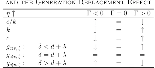
Table 1 displays the effects of conspicuous consumption for important economic

vari-ables.

TABLE 1

Steady State Effects of Conspicuous Consumption, and the Generation Replacement Effect

η↑ Γ<0 Γ = 0 Γ>0

c/k ↑ = ↓

k ↓ = ↑

c ↓ = ↑

gc(v,.) : δ < d+λ ↓ = ↑

gc(v,.) : δ =d+λ = = =

gc(v,.) : δ > d+λ ↑ = ↓

It has been frequently argued that one factor causing the low savings rates seen in

developed countries may be “overconsumption” resulting from a keeping up with the

Joneses consumption externality. This argument is not supported by representative

agent models, as argued above. The results of Wendner (2007) and Fisher et al. (2009)

are consistent with this argument, in the sense that they find conspicuous consumption

to raise the average propensity to consume out of accumulated wealth. In their models,

labor productivity is constant with age. Considering a declining labor productivity (or

gradual retirement), however, reveals that the impact of conspicuous consumption on

the propensity to consume (on savings) is ambiguous. Thus, on theoretical grounds,

as displayed by Table 1, there isno reason to believe that the consumption externality

has no impact on the steady state allocation. At the same time, there is no reason

to believe that the consumption externality would necessarily rise the propensity to

consume out of total wealth. In this sense, conspicuous consumption does not explain

the observed high propensity to consume (or low savings rates) on grounds of economic

the propensity to consume.

There are two implications. First, conspicuous consumption is a candidate for

explaining low savings rates observed in developed countries. The matter, however, is

an empirical one. Second, it is not clear at all that the propensity to consume, implied

by conspicuous consumption, is higher than optimal. Whether or not conspicuous

consumption leads to overconsumption is a different matter and is discussed in the

proceeding section.

4

Distortionary Effects and Optimal Taxation

In the following, we first first characterize an optimal steady state allocation. Next, we

show that the optimal allocation can be decentralized by an unfunded social security

system. Finally, we investigate how conspicuous consumption affects the optimal tax

scheme. Throughout, a tilde refers to an optimal value.

4.1

Optimal Allocation

In analogy to Calvo and Obstfeld (1988), the time-consistent utilitarian social welfare

function must take the form:

W(t) =

Z t

−∞

L(v, t)U(v, t)e−ρ(t−v)_e−ρ˜(v−t)_{d v +}

Z ∞

t

L(v, v)U(v, v)e−ρ˜(v−t)_{d v .}

The planner’s objective, at timet, is the sum of two components. First, the integral of

the expected remaining lifetime utilities of all cohorts alive at time t, measured from

the perspective of his and her birthdate.13 _{Second, the integral of the lifetime expected}

utilities of each of the generations to be born, as measured from the respective time

of birth. The planner’s discount rate, ˜ρ, needs not equal an individual’s pure rate of

time preference.

Consider L(v, t) = b eb v−d t_{, L(v, v) = b e}n v_{, n = b−d = 0, and change the order}

13_{The factore}−ρ(t−v)

of integration:

W(t) =

Z ∞

t

½Z s

−∞

b u[c(v, s), x(v, s)]e−[b+(ρ−ρ˜)] (s−v)d v

¾

e−ρ˜(s−t)d s . (24)

The planning problem consists of maximizing (24) by choosingc(v, s) andc(s) subject

to c(s) ≡ Rs −∞ b e

−b(s−v)_{c(v, s)dv and (15), where the planner considers the impact}

of consumption on the reference level according to (5). The (constrained) optimal

control problem is discussed in the appendix. Differential equations (43)–(46) yield

the following optimal steady state allocation, which is given by ˙c= ˙k = 0:

˜

r(k) = ˜ρ , (25)

c=y(k)−δ k . (26)

˙

c(v, .)

c(v, .) = ˜

ρ−ρ

˜

σ ,

cv(v, t) c(v, t) =−

˜

ρ−ρ

˜

σ . (27)

Equation (25) represents the Keynes-Ramsey rule for capital accumulation, and 26

restates the steady state resource constraint. Equations (27) show both the optimal

intragenerational and intergenerational consumption growth rates. In case the private

and social discount rates are equal, it is optimal to implement an egalitarian plan,

according to which every generation receives the same amount of consumption at any

given point in time. If, however, the private discount rate exceeds the social discount

rate, it is optimal to shift resources (consumption) towards the young cohorts, and

the intergenerational growth rate, cv(.)/c(.) is positive. If the private discount rate

is lower than the social one, the intergenerational growth rate is negative. As a

consequence, according to (27), individual optimal consumption rises (declines) with

age when private discount rate is lower (higher) than the social discount rate.

Two properties of the optimal allocation are particularly noteworthy. First,

con-spicuous consumption does not affect optimal average consumption and capital levels.

But the consumption externality affects the intergenerational and the

intragenera-tional consumption growth rates.

Second, in contrast to the market equilibrium, optimal consumption levels and

there is no GRE, and — in contrast to the market framework — the consumption

externality does not have an impact on the optimal allocation via the generation

replacement effect.

4.2

Decentralization and the Optimal Tax Scheme

In this and the proceeding subsections we show that the optimal steady state allocation

can be decentralized. The government applies two instruments: a constant tax on

capital income, τk, and lump sum transfers τ(v, t) > 0 and taxes τ(v, t) < 0. The

tax on capital income is motivated by two facts. First, conspicuous consumption

affects the propensity to consume out of accumulated wealth (the propensity to save)

in the market framework, while it does not affect the propensity to consume out of

accumulated wealth in the command optimum. Second, in the presence of conspicuous

consumption, the previous literature shows that a capital income tax is required to

decentralize the optimal allocation, once ˜ρ6=ρ (Abel, 2005).

Augmenting the market framework of Section 2 with the two instruments makes

necessary the following two modifications. First, the rate of interest is replaced by

the after tax rate of interest ˆr(t) = r(t) (1−τk). Second, the flow budget constraint

becomes:

˙

a(v, t) = ˆrA(t)a(v, t) +w(v, t) +τ(v, t)−c(v, t), (28)

where ˆrA_{(t) ≡ rˆ(t) + d. Define the present value of the future lump sum}

transfer-/tax stream by: β(v, t)≡R∞

t τ(v, t)e

−RˆA_(t,s)

, where ˆRA_(t

0, t1)≡

Rt1

t0 ˆr

A_{(s)d s. In the}

following, we refer such a lump sum scheme as a “transfer stream.” It follows:

Z ∞

t

c(v, s)e−RˆA(t,s)ds=a(v, t) +h(v, t) +β(v, t), (29)

c(v, t) = ∆−1[a(v, t) +h(v, t) +β(v, t)], (30)

c(t) = ∆−1[a(t) +h(t) +β(t)], β(t)≡

Z t

−∞

l(v, t)b(v, t)d v , (31)

where the propensity to consume, ∆−1_{, now involves the after tax rate of interest.}14

14_{Likewise, the transversality condition shown in footnote 5 also involves the after tax rate of}

Following the same procedure as in Section 2 yields:

˙

c(t)

c(t) = ˆ

r(t)−ρ

σ +

˜

σ σ

"

λ−(b+λ) ∆−1 k(t) +β(t)−

b

b+λβ(t, t) c(t)

#

= rˆ(t)−ρ

σ +

˜

σ σ

"

λ−(b+λ)k(t) +β(t)−

b

b+λβ(t, t) k(t) +h(t) +β(t)

#

(32)

˙

k(t) =y(t)−c(t)−δ k(t), (33)

˙

c(v, t)

c(v, t) = ˆ

r(t)−ρ

˜

σ +

˜

σ−σ

˜

σ

˙

c(t)

c(t),

cv(v, t) c(v, t) =−

ˆ

r(t)−ρ

˜

σ . (34)

Except for the public sector’s instruments, these equations of motion are identical to

those given in Section 2. The capital accumulation equation (33), however, deserves

a comment.

In general, a household’s flow budget constraint involves transfers and taxes,

τ(v, t), which show up at the aggregate capital accumulation equation if and only if

the government does not run a balanced budget. Here, we argue that the government

can run every feasible transfer scheme such that the government budget is balanced

period by period. A balanced budget at date t implies: Rt

−∞ l(v, t)τ(v, t)d v = 0.

Consequently, the transfer scheme does not affect the capital accumulation equation,

once the budget is balanced period by period.

To see that every feasible transfer scheme can be implemented with a balanced

government budget, notice that — with no initial debt at t — the intertemporal

government budget constraint requires:

Z t

−∞

l(v, t)β(v, t)d v+

Z ∞

t

b β(s, s)e−Rˆ(s,t)_{d s = 0. (35)}

It can easily be shown that, as preferences are monotone, the intertemporal

govern-ment budget constraint holds as a consequence of Walras law (Calvo and Obstfeld,

1988). Its main interpretation is that the present value of all present and future

primary deficits equals zero (otherwise the transfer scheme is not feasible).

Considerany given feasible transfer scheme, and define the date-s-primary deficit

π(s) ≡ Rs

−∞ l(v, s)τ(v, s)d v, where possibly {π(s)}∞s=t 6= 0. Consider the expected

future transfer stream of an agent born at date t, {τ(t, s)}∞

her transfer stream. The expected value of the transfer stream does not change due

to the fact that the present value of primary deficits is zero. Thus, β(t, v) is not

affected, but the transfer scheme now involves a balanced budget period by period

(Calvo and Obstfeld, 1988). In the following we only consider transfer schemes that

involve balanced budgets.

The two government instruments serve specific purposes. The capital income tax

is capable of correcting the intergenerational consumption growth rate. The lump

sum tax/transfer-scheme is capable of correcting the average capital level.

4.3

Capital Income Tax

It is shown below, that the transfer scheme is indeed capable of correcting for the

average capital level. Given that the optimal capital level can be decentralized by the

transfer scheme, the function of the capital income tax is to adjust the

intergenera-tional consumption growth rate, cv(.)/c(.).

For the following proposition, we assume that, in the steady state,k = ˜k resulting

from an optimal transfer scheme. That such a tax/transfer system exists (and which

properties it has) is shown in the following subsection.

Proposition 4 (Optimal Capital Taxation) Suppose k = ˜k by an optimal

trans-fer scheme. Then it is not optimal to tax capital income in the steady state, in spite

of a consumption externality.

Proof. Considering (27) and (34), optimality requires ˆr = ˜ρ. That is ˆr = r(˜k)(1−

τk) = ˜ρ(1−τk), which equals ˜ρ only withτk = 0. ||

The fact that the consumption externality affects the intergenerational consumption

growth rate does not justify a tax on capital income in the long run.15 _{This result}

is in contrast to Abel (2005), who shows that, in general, conspicuous consumption

15_{Erosa et al. (2002), Mathieu-Bolh (2006), and Spataro et al. (2008) show that optimal steady}

gives rise to a nonzero optimal tax rate on capital income. The capital income tax is

required to adjust the intergenerational consumption growth rate.

The fact that Proposition 4 differs from the results shown by Abel (2005) is

ex-plained as follows. The propensity to consume is age-dependent in the two-period

OLG model of Abel (2005), while it is independent of age in the continuous time OLG

model. Decentralization of the optimal allocation requires lump sum taxes and

trans-fers (as discussed below). Implementation of an optimal lump sum transfer scheme

transfers wealth across generations, which affects a household’s propensity to

con-sume — thereby the intergenerational consumption growth rate — in the two-period

OLG model. As a consequence, an additional instrument (the capital income tax)

is required to restore the optimal intergenerational consumption growth rate. This

mechanism is not at work in a continuous time OLG economy. Implementation of

an optimal lump sum transfer scheme transfers wealth across generations, but it has

no impact on the propensity to consume. Therefore no further instrument to correct

for the impact of a lump sum transfer scheme on the intergenerational consumption

growth rate is needed.

4.4

Unfunded Social Security System

We now show that the optimal allocation can be decentralized by a lump-sum transfer

scheme with the capital income tax rate being at its optimum (τk = 0). Considering

the equations of motion describing a market equilibrium, (32) – (34), we focus on

a characterization of β(t, t) and β(t) in the steady state. To simplify notation, let

β0 ≡β(t, t), and β ≡β(t), in a steady state.

Without loss of generality, we consider balanced budget lump-sum transfer schemes

only. It is important to note that a balanced budget scheme does not imply β = 0.

We will distinguish schemes according to the following definition.

Definition 2 (Unfunded Social Security) A balanced budget lump-sum transfer

scheme is said to be an unfunded social security system (U) if β0 < 0 and β > 0.

security system (RU) if β0 >0 and β <0.

If the optimal lump-sum transfer scheme distributes wealth away from the elder

co-horts towards the young coco-horts we refer to the scheme as a reverse unfunded social

security system.

Walras law implies the intertemporal government budget constraint, which can be

rewritten as: β+β0

R∞

t b e−R(t,v)d v= 0. In a steady state:

β0 =−

˜

ρ

b β . (36)

Thus, any balanced budget lump-sum transfer scheme is either anU scheme or aRU

scheme. In the appendix, β is derived. It follows:

b

˜

ρβ0 =

µ

1 ˜

ρ+d+λ −

1 ∆−1

¶

(y−δ k) + d+λ ˜

ρ+d+λk , (37)

which allows to (i) distinguish aU scheme from aRU scheme, and (ii) find the effects

of conspicuous consumption on the optimal transfer scheme.

The first result of this subsection concerns to the sign ofβ0.

Proposition 5 (Unfunded Social Security scheme) The optimal social security

scheme is a U scheme (is a RU scheme) if:

sgn

·

Γ +ρ˜−ρ ˜

σ

¸

>0

µ

sgn

·

Γ + ρ˜−ρ ˜

σ

¸

<0

¶

.

Proof. See appendix.||

If the pure rate of time preference equals the social discount factor, the sign of β0

is fully determined by the sign of the GRE: sgnβ0 = −sgn Γ. In the standard case

with λ = 0 (that is, Γ < 0), the proposition implies: β0 > 0. Consequently, it is

optimal to implement a reverse unfunded social security scheme. Cohorts are faced,

at birth, with a declining transfer stream. Thus, consumption smoothing requires

them to (initially) lower consumption levels and rise savings. Consequently, the RU

system raises capital accumulation to the point at which k = ˜k.

Proposition 5 also identifies two necessary conditions for a U transfer scheme

is optimal to redistribute towards the old cohorts if their labor productivity declines

strongly enough with age (λ >λ˜). Second, if Γ≤0, ˜ρ > ρ by a sufficient amount. In this case, it is optimal to implement a transfer of resources towards the old cohorts,

as their socially optimal consumption is higher than that of the young cohorts.16

Effects of Conspicuous Consumption. If Γ 6= 0, conspicuous consumption affects k

in the market economy (according to Proposition 1), while it leaves unaffected k in

the command optimum. Based on this observation, one could expect conspicuous

consumption to rise β0 if Γ <0, and to lower β0 if Γ >0. The opposite, however, is

the case, as shown by Proposition 6. In the following we restrict our analysis to the

case: ˜ρ=ρ.

Proposition 6 (Unfunded Social Security and Conspicuous Consumption)

If Γ6= 0, conspicuous consumption affects the optimal unfunded social security system in the following way:

Γ_≷0⇒ ∂ β0

∂ η ≷0.

If Γ = 0, conspicuous consumption has no impact on the optimal unfunded social

security system.

Proof. See appendix. ||

Proposition 6 says that conspicuous consumption always reduces the decline or

in-crease (with age) of a cohort’s transfer stream. For example, if Γ < 0, β0 > 0 but

β <0. That is, the transfer stream decreases with age (and becomes negative,

even-tually). According to the proposition, conspicuous consumption lowers the rate of

decline in the transfer stream.

This counterintuitive “smoothing effect” has the following intuition. Consider a

transfer scheme which fully decentralizes the optimal allocation. A rise in the strength

of conspicuous consumption (of η) has no effects on the socially optimal average

consumption and capital levels. If, for example, Γ <0, both the average consumption

16_{A special case is given by Γ = 0, in which case sgnβ}

and capital levels decline in a market economy. As c is directly proportional to the

average transfer stream, β has to be raised in order to restore optimality. The rise in

β requires a decline in β0, by (36). Intuitively, the consumption externality leads to

a decline in the laissez-faire average consumption level. A lowering in β0 lowers the

“initial” consumption level of a newborn cohort, and it raises its savings. Eventually,

in a steady state, the lowering inβ0 (the rise inβ) leads to increases in individual and

average consumption levels.

Proposition 6 has two important implications. First, a rise in the strength of

the consumption externality implies a “smoothening” (a lower rise or decline with

age) of the optimal transfer scheme. Second, the proposition shows that conspicuous

consumption introduces a distortion whenever Γ 6= 0. The result is noteworthy, as the consumption externality introduces a steady state distortion even for the case of

exogenous labor supply. Clearly, this result does not hold in a representative agent

economy, where — by definition — Γ = 0.

Whether or not the distortion leads to overconsumption, however, is a different

matter. We showed that the consumption externality implies steady state

overcon-sumption only if Γ>0, and it implies underconsumption if Γ<0.

5

Conclusions

Economists have been interested in conspicuous consumption for centuries.

Fre-quently, economists refer to conspicuous consumption as one factor for explaining

the low savings rates faced by many developed countries. Motivated by this

argu-mentation, this paper addresses two main questions. First, how does a “keeping up

with the Joneses” consumption externality affect consumption and savings decisions?

In more coarse terms, do people consume too much as a consequence of the desire to

keep up with the Joneses? Second, compared to a social optimum, does conspicuous

consumption lead to a distortion (to overconsumption)?

In the paper, we show that conspicuous consumption doesnot, in general, give rise

overconsump-tion according to a utilitarian social welfare funcoverconsump-tion. For both quesoverconsump-tions raised, the

sign of the generation replacement effect (present in an OLG model but absent in an

infinitely lived agent model) is identified to play a decisive role. The generation

re-placement effect refers to the difference between average and individual consumption

growth rates, which is based on the fact that individual consumption levels change

with age.

In the absence of the generation replacement effect (GRE), conspicuous

consump-tion does not have an impact on consumpconsump-tion or savings decisions. In its presence,

however, conspicuous consumption raises (lowers) the steady state propensity to

con-sume out of total wealth if individual consumption growth is positive (negative).

Individual consumption growth is positive if individual labor productivity does not

decline “by much” with age (in which case the GRE has a negative sign). Individual

consumption growth is negative if individual labor productivity declines “strongly”

with age (in which case the GRE has a positive sign).

Along the same line, the steady state effects of a consumption externality are shown

to be distortionary only in the presence of a GRE. If the GRE is negative the keeping

up with the Joneses consumption externality implies steady state underconsumption.

Only if the GRE is positive (the rate of individual labor productivity decline is large

enough), does the consumption externality lead to steady state overconsumption.

These results have important implications. First, it is generally mistaken to

as-sociate conspicuous consumption with an increase in the propensity to consume or

with overconsumption. Both might happen. But while the former happens in case

the GRE is negative (for a low rate of individual labor decline), the latter happens

in case of a positive GRE (for a high rate of individual labor decline). As a

conse-quence, overconsumption requires a decline in the propensity to consume due to the

consumption externality.

Second, the consumption externality does not give rise to a positive capital income

tax rate in the long run. The main reason is that the propensity to consume is

Third, the market equilibrium can be decentralized by a social security system.

The paper identifies the sign of the GRE to determine whether the scheme is an

unfunded social security scheme or a reverse unfunded social security scheme (with

transfers from the old to the young). Unless the labor productivity declines strongly

enough with age, the optimal scheme turns out to be a reverse unfunded social

se-curity scheme. Finally, a rise in the strength of the consumption externality implies

a “smoothening” (a lower rise or decline with age) of the optimal unfunded social

security transfer scheme.

Given the theoretical findings of this study, it is important to empirically identify

the sign of the GRE appropriately. In this sense, I hope that this study helps to clarify

the effects of conspicuous consumption, and it will contribute to the future debate of

the effects of consumption externalities in a dynamic framework.

Appendix

A.1 Derivation of Individual Consumption. For any individual, consider the

current value Hamiltonian:17

Hc[c(v, s), a(v, s), µa(s), s] =u(c(v, s), x(v, s))+µa(s)[(r(s)+d)a(v, s)+w(v, s)−c(v, s)].

For all s≥t,c(v, s) is chosen such as to maximize expected utility (7), subject to:

c(v, s)≥0,

˙

a(v, t) = (r(s) +d)a(v, s) +w(v, s)−c(v, s), a(v, t) given, lim

s→∞ µa(s)e

−(ρ+d)s_{a(v, s) = 0.}

From ∂ Hc/∂ c(v, s) = 0 and −∂ Hc/∂ a(v, s) = ˙µa−(ρ+d)µa, it follows:

µa(s) = uc(v,s) =

c(v, s)−σ

1−η

·

c(s)

c(v, s)

¸σ˜−σ

, (38)

gc(v,s) ≡

˙

c(v, s)

c(v, s) =

[r(s)−ρ] ˜

σ +

˜

σ−σ

˜

σ

˙

c(s)

c(s),

17_{Notice thatη < σ, which is sufficient for the Hamiltonian to be concave in the decision and state}

where no individual considers its impact of individual consumption on the reference

level. Thus,

c(v, s) =c(v, t)e

Rs t

[r(s)−ρ] ˜

σ +

˜

σ−σ ˜

σ

˙

c(s)

c(s)d s_.

Combining this equation with the intertemporal budget constraint (16), and

consid-ering the definition of ∆(t) in (17) yields: c(v, t) = ∆−1(t) [a(v, t) +h(v, t)]. ||

A.2 Proof of Lemma 1

(i) Restate the average consumption growth rate as:

˙

c(t)

c(t) = ˙

c(v, t)

c(v, t) −b

c(t)−c(t, t)

c(t) ,

where we consider the fact ˙c(t) = b c(t, t)−b c(t)+gc(v,t)c(t). Taking (22) into account:

Γ(t) = b[c(t, t) − c(t)]/c(t), that is, Γ(t) = 0 ⇐ c(t, t) = c(t) ⇔ ∆−1_{h(t, t) =}

∆−1_{[h(t) +a(t)]⇔h(t, t) =h(t) +a(t). Also, Γ(t) = 0⇐b= 0. |}

(ii) If b >0 and λ= 0, h(t, t) =h(t)< h(t) +a(t)⇔c(t, t)< c(t)⇔Γ(t)<0.|

(iii) From the definition of Γ(t), it directly follows that ˜λ(t) = b k(t)/h(t). Ceteris

paribus, ∂Γ(t)/(∂ λ) =h(t)/[h(t) +k(t)]>0. ||

A.3 Figure 1. The figure displays two demarcation lines in (k, c) phase space: ˙k = 0,

and ˙c= 0.

The k˙ = 0 line. We define the graph of ˙k = 0 by the set kk ≡ {(k, c) ∈ R2+|c =

y(k)−δ k}. Asy(0) = 0, (0,0)∈kk. Next,∂ c/∂ k >0 as long asy′_{(k)−δ=r(k)>0,}

and ∂ c/∂ k < 0 when r(k) < 0. As y(k) is strictly concave, and (−δ k) is weakly concave, y(k)−δ k, that is, the ˙k = 0 line, is strictly concave. The capital stock for which r(k) = 0 is denoted the “golden rule” capital stock in Figure 1: r(kGR) = 0.

Finally, for the maximal attainable stock of capital, kmax, it holds: y(kmax) = δ kmax.

For any given (k, c), a rise in λ clearly lowers y and tilts the ˙k = 0 line clockwise

down. It lowers both kGR and kmax.

The c˙ = 0 line. From (M.SS.1) it follows:

c=k (b+λ)[(r+d) ˜σ−(r−ρ)]