Adaptive Nonlinear Filter using Main Texture Direction for Mixed Noise in Color Image Processing

2016 International Congress on Computation Algorithms in Engineering (ICCAE 2016) ISBN: 978-1-60595-386-1

1 INTRODUCTION

During the image acquisition, signal amplification and transmission, which are often corrupted by different types of noise, the most noise is Additive Gaussian noise and impulse noise [1-4], both of them have significantly influenced the image processing. Filtering noise and preserving the image features from the corrupted images are important parts of image pre-treatments. Many filters have been proposed for the removal of the noise. For instances, the classical standard median filter (SMF), the switching bilateral filter (SBF) [5], the high performance filter (HPF) [6], the spatially adaptive denoising algorithm (SADA) [7] and the new method for removing mixed noises (MNF)

[8]

, although these filters can remove the noise effectively, they fail to preserve image features and have higher computational complexity, like MNF and SBF.

To address above problems, in this paper, a novel adaptive nonlinear filter (ANF) using main texture direction is proposed for the removal of mixed noise in corrupted color images processing, which is motivated by the theory of the Chebyshev’s theorem, and the fuzzy mean process is used to estimate

adaptively parameters of detector; for the filter, since the Radon transform has stronger robustness to various noises, the local features of the image are gained by developing the local texture direction probability density distributions, on which the Radon transform is performed. The performance of ANF is quantitatively measured by the important parameters. Moreover, the advantages of the ANF are demonstrated on test images at various types of noise corruption, and the results are compared both visually and quantitatively with SMF, SBF, HPFSM, SADA and MNF. Extensive experimental results show that the ANF outperforms these other filters. Moreover, the ANF achieves excellent performance for filtering high-density salt-and-pepper noise, random-valued impulse noise, Gaussian noise and many types of mixed noise. Simultaneously, the ANF has very low computational complexity, the average time of the ANF being only 1.69s, whereas SBF was 529.04s, HPFSM was 13.40s, SMF was 5.27s, SADA was 3.33, and MNF was 5220.20s.

The rest of this paper is organized as follows: the ANF is described in Section 2; Section 3 presents experimental results; finally, Section 4 concludes this paper.

Adaptive Nonlinear Filter using Main Texture Direction for Mixed

Noise in Color Image Processing

Xueqing Zhao*1, Meihong Shi1, Xin Shi1 & Haris Iskandar Loh Bin Abdullah2 1

College of Computer Science, Xi'an Polytechnic University, Xi’an, Shaanxi, China

2

College of Graphic Design, RIMA College, Malaysia

ABSTRACT: Adaptive nonlinear filter (ANF) using main texture direction is proposed for the removal of mixed noise from corrupted color images processing. The purpose of this work is to focus on designing noise detector and noise filter. For the detector, Chebyshev’s theorem and the fuzzy mean process are used to estimate adaptive parameters of detector; for the filter, the authors use the local texture direction probability density distributions which are gained by performing the Radon transform of the image. Extensive experimental results show that the proposed ANF outperforms other filters in terms of important evaluation metrics; in particular, the computational complexity of the ANF is much lower than the test filters.

Keywords: mixed noise; adaptive nonlinear filter; Chebyshev’s theorem; radon transform; color image processing

2 PROPOSED ADAPTIVE NONLINEAR FILTER

2.1 The main texture direction of the image

The Radon transform is widely used in imaging processing, and it is suited for line parameters extraction even in noise corrupted images [9]. In this paper, we use the Radon transform to determine the texture information of the main texture direction of the image. A two-dimensional (2-D) Radon transform of a 2-D object defines 1-D line integrals in the projection space, and the object of the Radon transform is defined in (1):









  



 ( ) ( cos sin , sin cos ) )

,

( _    

R (1)

Where: f (x, y) is a 2-D function; Gθ(ρ) is periodic in

θ with a period of 2π and is symmetric; ρ and ζ form a rotated coordinate system with an angle θ with respect to the x-y coordinate system.

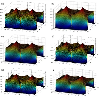
Figure 1 shows a visualization of the main texture direction of Radon transform on log of Fourier

spectrum on the test image Lena (256×256), we can see that salt-and-pepper noise, Gaussian noise, random-valued impulse noise, salt-and-pepper with random-valued impulse noise, and salt-and-pepper with Gaussian noise have no effect on the image after Radon transform, moreover, it also shows that the main texture direction by Radon transform has a much stronger robustness [see Figure 1(b)-(f)].

2.2 Noise detector

In statistical theory, only the average and the standard deviation of the statistical data are known. Chebyshev found that the number of observations was at least (1-k-2_{)% in the k-standard deviation of the distance}

near the average [6, 10]. The statement of this observation is described in Chebyshev’s theorem: The probability that any random variable X will set a value within k standard deviations of the mean is at least 1-1/k2, that is:

P(μ-kσ<X<μ+kσ)≥1-1/k2 ₍₂₎

(b) (a)

(c) (d)

(e) (f )

Figure 1. Radon transform of the Fourier spectrum of Lena image (horizontal axes shows the texture direction θ of the image, and vertical axes shows main texture direction): (a) the original Lena image, (b) adding in 20% salt-and-pepper noise, (c) adding in (0.2, 0.5) Gaussian noise, (d) adding in 20% random-valued impulse noise, (e) adding in 20% random-valued impulse

Where: μ and σ are respective the mean and standard deviation of the observed data. The interval of the observed data is [μ-kσ, μ+kσ]. According to the Chebyshev’s theorem, we design a noisy detector of the ANF, and we define it as follows:

1) /( ) , ( 2 2 A ) , (    



g (3)

And the standard deviation is shown as follows:

τ

k1/ 1 (4) Where a filter window of size w×w and g(i, j) is the intensity value at the (i, j)-pixel location, two sets A and B are defined as follows:













           w w w w gi s j t

t j s i g A (5)













2 / 1) ( 0, 0 t 0,

s ( , )

) , (          

 w w

w w t j s i g t j s i g B (6)

From the inherent properties of the Radon transform, we can estimate the local texture direction probability density distribution to capture the directional information of the image. According to Equation (1), the Radon transform along the texture principal direction has larger variations. Given angle θ, the variation σθ along the line defined by θ is defined as

follows:

γ

γ θ

θ(



 ₍₇₎

Where: Nγ is the total number of the angle, and μθ

represents the mean value of p(r, θ), that is to say:

γ γ

θ(



 ₍₈₎

The local texture direction probability density distribution can be determined from 



     ) / ( p .

0 20 40 60 80 100 120 140 160 180 200

4 4.5 5 5.5 6 6.5 7 7.5

8 x 10

-3

The angle X: 180 Y: 0. 0070

X: 135 Y: 0. 0047 X: 90 Y: 0. 0064 X: 45

Y: 0. 0060 X: 0

Y: 0. 0070

0 20 40 60 80 100 120 140 160 180 200

4 4.5 5 5 .5 6 6.5 7 7.5

8x 10

-3

The angle X: 180 Y: 0. 0069

X: 135 Y: 0. 0048 X: 90 Y: 0. 0065 X: 45

Y: 0. 0060 X: 0

Y:0. 0069

0 20 40 60 80 100 120 140 160 180 200

4 4. 5 5 5.5 6 6 .5 7 7.5

8x 10

-3

The angle X: 180 Y: 0. 0067

X: 135 Y: 0. 0051 X: 90 Y: 0. 0066

X: 45 Y: 0. 0057 X: 0

Y: 0. 0067

P ro b a b il it y d e n si ty P r o b a b il it y d e n si ty P r o b a b il it y d e n si ty

0 20 40 60 80 100 120 140 160 180 200

4 4.5 5 5.5 6 6.5 7 7.5

8x 10

-3 The angle P ro b a b il it y d en si ty

0 20 40 60 80 100 120 140 160 180 200

4 4.5 5 5.5 6 6.5 7 7. 5

8x 10

-3

The angle X: 180 Y: 0. 0067

X: 135 Y: 0. 0052 X: 90 Y: 0. 0066

X: 45 Y: 0. 0056 X: 0 Y: 0. 0067

P ro b a b il it y d e n si ty

X: 0 Y: 0. 0069

X: 45 Y: 0. 0060

X: 90 Y: 0. 0064

X: 135 Y: 0. 0047

X: 180 Y: 0. 0069

0 20 40 60 80 100 120 140 160 180 200

4 4.5 5 5.5 6 6.5 7 7.5

8x 10

-3 The angle P ro b a b il it y d en si ty X: 0 Y: 0. 0068

X: 45 Y: 0. 0059

X: 90 Y: 0. 0065

X: 135 Y: 0. 0049

X: 180 Y: 0. 0068 (a)

(c)

(b)

(d)

(e) (f )

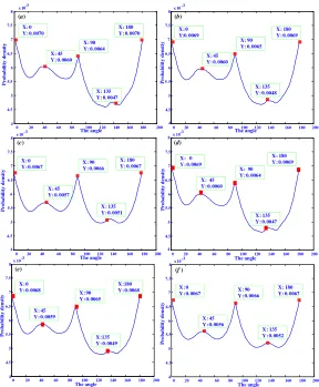
Figure 2. Main texture direction of Lena determined by Radon transform (horizontal axes: θ angle; vertical axes: probability density): (a) the original image, (b) adding in 20% salt-and-pepper noise, (c) adding in (0.2, 0.5) Gaussian noise, (d) adding in

Figure 2 shows the main texture direction of one of the test images Lena (256×256) determined by applying the Radon transform. We can see that salt-and -pepper noise, Gaussian noise, random-valued impulse noise, salt-and-pepper with random-valued impulse noise, and salt-and-pepper with Gaussian noise have no effect on the image after Radon transforming, and this method has a much stronger robustness.                 

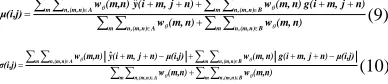
m n,(m,n)A m n,(m,n)B m n,(m,n)A m n,(m,n)B

n) (m, w n) (m, w n) j m, g(i n) (m, w n) j m, (i y (m,n) w μ(i,j)     ˆ (9)                   

m n,(m,n)A m n,(m,n)B m n,(m,n)A m n,(m,n)B

(m,n) w (m,n) w μ(i,j) n) j m, g(i n) (m, w μ(i,j) n) j m, (i y (m,n) w σ(i,j)     ˆ (10)

Where wθ(m,n) denotes the local weight which is

computed from the local texture direction probability density: ) ( ) , ( 

 mn p

w  (11)

In fact, according to the experimental results, the probability density values of the local texture-direction are the same for the angle pairings θº and θº+180º, thus, we just consider θ{0º, 45º, 90º, 135º, 180º}.

To remove noise in corrupted images, we use the fuzzy mean process to adaptively estimate parameters. This process performs the fuzzy mean of input variables F_mean by adopting the trapezoidal function as the membership function [11]. The membership degree is usually a value in the range [0, 1], where “1” denotes full membership and “0” denotes no membership. Equation (12) is defined by the parameter set F_mean =[0, α, β, 255]:

                   255 0 255 255 255 1 0 0 0 x x x x x x x x

fF mean

, ), /( ) ( , , / , ) ( _       (12)

Hence, according to the local standard deviation σ(i, j) in the scanning window, the local area E(i, j) is defined: mean F f j i j i

E(, )(, )/ _ (13)

Where δ represents a constant; fF_mean denotes the

relation degree of the local pixels in the observed window, which is produced adaptively by the fuzzy mean process. So the noise determining function D(i,j) is defined by the local features of the image given in (9) and (13). It can be written as follows:

        wise other j) E(i j) μ(i j) j) or y(i E(i j) μ(i j) if y(i j i D 0

1 , , , , , ,

) ,

( (14)

Where ‘1’ signifies a noisy pixel and ‘0’ means a noise-free pixel.

2.3 Adaptive nonlinear filter The ANF is defined in (15):

                     erwise oth y(i,j), i,j) , if D( G(m, n)

G(m, n)

n) m, j i G(m, n) g( n) m, j (i y G(m,n) (i,j)

y m n,(m,n) A m n,(m,n) B m n,(m,n) A m n,(m,n) B

1

ˆ

ˆ ₍₁₅₎

Where G(m, n) is the modified Gaussian filter, which is used to handle the degree of local smoothness

[12]

, and it is defined in (16). The algorithm of the ANF is described in Table 1.

) 1 ) , ( / ) )( , ( exp( ) ,

(_{i j  } 2_{i j i}2_j2 _{i j }

G   (16)

Table 1. The algorithm of the ANF.

Steps The algorithm of the ANF

Step1 Input: the noisy image y with the size of M×N.

Step2

For each pixels in the noise image, set up two process sets A and B according to (5) and (8) respectively.

Step3

Determine whether the current pixel g(i, j)is a noisy or noise-free.

1)According to the Chebyshev’s theorem, compute the parameter k by (3) and (4). 2)Solve the local weight from the local texture direction probability density using (11). 3)Estimate the local weighted mean μ from (9).

4)Estimate the local standard deviation σ using (10).

5)Determine parameters α and β of the fuzzy mean process.

6)Use the noise-determining function of (15) to detect the noise in the image.

Step4

Filter the noisy pixels.

1)According to the modified Gaussian filter in (16), the degree of local smoothness can be calculated.

2)The noisy pixels are removed using the proposed filter function of (15).

Step5 Output: the de-noised image yo.

3 EXPERIMENTAL RESULTS

Several parameters are used in the ANF. In Equation (13), the constant δ increases, and the bounds of the local area are looser, leading to higher noise detection error; tighter bounds result in loss of important details of the image. In our simulations, we take δ=0.0002. The parameters α and β that characterize fF_mean are

determined:

used to quantify image restorations. They are defined as follows:

) ) ( /

max

lg( '

, , ,

, _{ } 

 M

m N

n

n m n m n

m n

m I _MN I I

PSNR

1 1

2 2 1

10 ₍₁₈₎

   



 _

 _

 

Num I

I MSENS

M

m N

n ' m,n m,n ))/ (

( lg

1 1

2

10 ₍₁₉₎

Where Im,n and I´m,n denote the respective pixel

values of the original and denoised images, and Num is the number of noisy pixels in the original image. To demonstrate the advantage of the ANF, the performance of the ANF was tested under various noise corruptions, and the results are compared with the other filters SBF, HPFSM, SMF, SADA and MNF. The performances of all these filters were quantitatively measured using the aforementioned parameters.

Figure 3.The typical test images Lena, Girl and Airplane.

3.1 The capabilities of the restoration

Table 2 lists PSNR and MSENS of the ANF on the test images, Lena, Girl and Airplane, which are corrupted by the salt-and-pepper noise, the random-valued impulse noise, the Gaussian noise and various types of mixed noise. The better values of PSNR and MSENS are described in Table 2 with black font. From Table 2, we can see the ANF outperforms the other filters.

3.2 The capabilities of the detail preserved

To analyze detail-preserving capabilities of the ANF, three test images are degraded by various types of noise. Figure 4 shows the restored images, which are restored by the six filters: SBF, HPFSM, SMF, SADA, MNF and the ANF. From Figures 4(a)–(u), we note that the ANF gives a good visual image both in filtering the noise and preserving the image features

3.3 Computational complexity

To make a reliable comparison, each of these filters

run 50 times on a personal computer equipped with an Intel 1.86 GHz CPU and 1GB RAM memory, and the mean runtime is calculated. Table 3 shows the average computational time for various images, which presents obviously that the ANF takes much shorter execution time, and the computational complexity of the ANF is lower than other filters.

Figure 4. (a) cutout of the Lena image, corrupted with random-valued impulse noise (30%); (b) cutout of the Girl image, corrupted with mixed noise (Gaussian noise, υ=30%); (c) cutout of the Airplane image, corrupted with mixed noise (Gaussian noise, υ=60%); (d), (e), (f) filtering using the SBF; (g), (h), (i) filtering using the HPFSM; (j), (k), (l) filtering using the SMF; (m), (n), (o) filtering using the SADA; (p), (q), (r) filtering using the MNF; (s), (t), (u) filtering using the ANF.

Table 3.Results of the ANF on variousfiltered images.

Images Execution Time (Unit: s)

SBF HPFSM SMF SADA MNF ANF

Lena 224.56 6.78 2.13 1.58 2280.00 0.45

Girl 679.80 16.44 6.80 4.19 6658.99 2.34

Airplane 682.78 16.98 6.89 4.23 6721.46 2.29

Table 2. PSNR(dB) and MSENS results of the filtered images (Lena, Girl and Airplane) at different types of noise.

Noise Images

Filters

Noise level

SBF HPFSM SMF SADA MNF ANF

Salt& Pepper

noise

Lena

30% 26.72/152.26 10.61/4761.5 20.14/518.10 18.12/828.6 17.10/1207.3 20.02/535.28

60% 16.60/1293.40 7.41/9780.00 10.70/4594.5 14.10/2085.3 7.00/10133.0 16.10/1320.1

80% 9.00/6778.80 6.00/13152.0 7.00/10439.0 12.40/3079.7 6.00/12813.0 14.20/2041.8 90% 6.00/11503.0 5.98/14833.0 6.00/14509.0 11.70/3663.1 5.00/15946.0 13.40/2450.6

Girl

30% 27.16/108.28 10.8/4730.80 16.69/607.81 16.20/1351.6 12.50/3190.9 17.80/924.38

60% 15.00/1788.40 8.50/7926.80 10.00/5693.7 11.8/3778.5 7.00/10976.0 12.90/2974.9

80% 8.30/8354.50 7.00/10769.0 6.00/13163.0 9.80/6061.8 6.00/13285.0 10.70/4938.9 90% 6.98/12980.0 6.00/12701.0 5.00/17808.0 8.90/7425.2 5.00/15424.0 9.70/6122.2

Airplane

30% 22.80/336.90 9.00/7813.10 19.52/690.47 17.10/1198.7 13.10/2998.3 18.01/975.36

60% 14.70/2110.30 6.00/16911.0 10.70/5237.3 13.00/3087.9 7.00/11590.0 14.10/2419.9

80% 8.60/8504.70 5.00/21602.0 7.00/12202.0 11.10/4809.8 6.00/15391.0 12.10/3826.6 90% 6.00/13856.0 4.00/23412.0 6.00/16435.0 10.30/5730.9 5.00/16783.0 11.30/4576.2

Radom-valued

impulse noise Lena

10% 27.94/86.43 27.02/106.78 31.05/42.22 29.65/58.32 31.14/41.41 26.33/125.25 30% 22.75/285.42 22.23/322.00 23.08/279.44 23.00/269.36 23.14/261.33 23.34/268.61 60% 17.73/986.62 15.40/1558.4 17.20/1024.0 17.30/1006.8 17.00/1071.1 17.40/976.30 80% 15.00/1702.0 12.20/3244.4 14.80/1791.6 14.90/1759.4 14.60/1874.1 15.90/1526.8

Girl

10% 28.21/85.07 20.33/560.86 30.21/54.16 29.21/67.89 30.76/47.32 27.09/110.15 30% 23.02/281.05 19.12/728.57 23.08/277.14 22.63/307.71 23.29/264.12 23.54/253.53 60% 17.61/975.79 16.70/1024.3 17.40/1022.7 17.10/1089.1 17.20/1071.15 17.82/957.45 80% 15.20/1707.5 14.60/1989.2 15.00/1794.6 14.80/1879.3 14.70/1928.1 15.80/1680.4

Airplane

10% 23.87/260.01 25.58/183.77 27.32/114.54 25.79/163.24 29.05/77.71 23.08/308.71 30% 21.45/444.14 21.59/432.4 22.61/337.33 22.14/376.49 23.11/301.31 23.82/413.53 60% 17.40/1120.7 11.90/4036.5 17.60/1066.6 17.60/1080.6 17.40/1109.9 18.10/956.32 80% 15.40/1789.8 8.00/10957.0 15.60/1698.6 15.50/1754.1 15.50/1731.1 15.80/1575.3

Gaussian

noise

Lena

10% 28.68/72.89 23.91/218.47 30.88/43.91 30.64/46.45 31.03/42.38 27.12/104.25 30% 25.57/149.39 17.00/1027.1 23.85/222.06 24.76/179.53 22.33/314.51 25.96/136.38 60% 20.63/465.18 11.00/4306.0 18.42/774.81 20.32/499.61 19.64/584.95 23.31/250.86 80% 18.45/768.95 9.10/6643.20 16.20/1304.00 18.19/814.69 19.08/665.23 21.69/365.16

Girl

10% 29.08/65.59 20.55/506.26 30.22/54.06 29.85/58.39 31.02/49.35 28.01/89.10 30% 26.08/139.06 18.13/889.4 24.21/213.34 25.36/163.89 22.91/288.53 26.56/124.35 60% 21.38/410.04 13.30/2645.9 19.17/682.61 21.06/441.62 20.34/521.87 23.94/227.30 80% 19.26/669.20 11.30/4174.5 17.10/1104.00 19.09/695.46 19.86/583.28 22.29/332.92

Airplane

10% 24.29/237.51 24.98/197.10 27.42/112.04 26.21/148.46 28.60/86.37 23.42/286.18 30% 22.15/353.79 16.10/1511.4 23.13/299.75 23.58/270.42 21.56/430.46 22.93/318.75 60% 20.12/601.28 9.00/7813.56 18.65/840.19 20.20/578.80 19.21/739.19 21.59/430.66 80% 18.29/912.07 8.00/10957.0 16.70/1315.50 18.54/861.19 18.66/840.41 20.59/539.77

mixed noise Lena

Mixed1 26.99/107.45 14.30/2001.40 25.39/155.47 22.23/321.81 23.11/263.14 23.75/226.65 Mixed2 27.67/91.92 15.30/1606.70 29.29/63.26 22.66/291.47 25.34/157.44 23.51/239.75 Mixed3 27.58/93.90 24.14/207.39 28.79/71.11 28.52/75.73 28.89/69.39 26.18/129.83 Mixed4 20.09/526.97 12.90/2771.30 17.47/916.67 18.68/730.18 19.54/598.30 21.86/350.36 Mixed5 15.00/1698.20 7.80/9013.10 11.10/4147.70 14.20/2039.30 7.90/8723.50 16.00/1337.20 Mixed6 17.51/953.85 10.50/4845.70 16.50/1206.00 17.00/1072.00 16.60/1165.20 18.14/825.47

Girl

Mixed1 27.42/101.94 13.70/2403.50 25.56/156.68 21.38/410.76 23.38/258.74 23.08/277.67 Mixed2 28.27/83.88 14.30/2146.80 28.62/77.76 20.90/461.25 25.30/166.45 22.03/354.26 Mixed3 28.03/88.72 20.20/558.17 28.47/80.43 27.68/96.45 28.92/72.30 26.90/114.77 Mixed4 20.09/458.75 11.90/3632.80 18.26/841.76 18.60/778.43 19.95/569.96 21.51/397.99 Mixed5 14.80/1856.60 8.30/8317.20 10.30/5270.90 11.80/3803.60 7.00/9797.00 12.80/3010.00 Mixed6 10.20/5339.60 12.50/3185.60 16.70/1205.70 17.20/1074.70 16.80/1169.90 18.33/826.78

Airplane

Mixed1 23.60/275.20 14.30/2284.90 24.02/244.59 21.10/479.25 22.17/375.61 21.46/444.74 Mixed2 23.45/285.85 13.80/2570.50 26.01/155.47 25.44/176.87 24.08/244.14 21.91/403.43 Mixed3 23.92/256.33 23.92/253.64 26.45/140.09 26.45/159.46 27.34/114.64 23.02/312.53 Mixed4 19.62/657.31 8.0/10784.0 17.80/1013.60 18.53/863.45 18.98/779.01 20.31/576.68 Mixed5 13.80/2547.40 7.00/12325.0 11.00/4859.20 13.00/3063.40 8.00/10330.8 14.10/2403.30 Mixed6 17.60/1068.60 7.00/12424.0 17.30/1147.30 17.60/1077.10 17.11/1207.30 17.90/1009.70

 Various types of the mixed noise: Mixed1: Salt & pepper noise 10%, Gaussian noise 20%; Mixed2: Salt & pepper noise 10%,

4 CONCLUSIONS

In this paper, a novel ANF has been proposed for the removal of mixed noise from corrupted color images. This work has been accomplished by two stages: the noise detector and the noise filter. The theory of Chebyshev’s theorem and the fuzzy mean process has been used to design the detector; the Radon transform has been introduced to determine the texture direction probability density distributions of local areas of the image; local features of the image are combined to filter the noisy pixels. Extensive experimental results have shown that the ANF outperforms other filters both visually and quantitatively other filters. Moreover, the ANF has been confirmed to have very low computational complexity.

ACKNOWLEDGEMENT

This paper is sponsored by Doctoral Research Foundation of Xi'an Polytechnic University.

REFERENCES

[1] Mohan V M, Durga R K, & Devathi S, et al. 2016. Image Processing Representation Using Binary Image; Grayscale, Color Image, and Histogram[C]//Proceedings of the Second International Conference on Computer and Communication Technologies. Springer India: 353-361. [2] X.Q. Zhao, X.M. Wang & L.Ch. Zhang. 2012. Reaction

diffusion equation based image denoising algorithm, Chinese Journal of Electronics, 21(3): 495-499.

[3] X. Wang, X.Q. Zhao, F.X. Guo & J.F. Ma. 2011. Impulsive noise detection by double noise detector and removal using adaptive neural-fuzzy inference system, Aeu-international Journal of Electronics and Communi-cations, 65(5): 429-434.

[4] Mishra D, Bose I, & Das M, et al. 2014. Detection and reduction of impulse noise in RGB color image using fuzzy technique[M]//Distributed Computing and Internet Technology. Springer International Publishing: 299-310. [5] Ch. H. Lin, J. Sh. Tsai & Ch. T. Chiu. 2010. Switching bilateral filter with a texture/noise detector for universal noise removal, IEEE Transactions on Image Processing, 19(9): 2307-2320.

[6] P.T. Yu, Y.L. Chen & B.M. Chang. 2008. A high performance filter based on statistic methods for image processing, Proc. of International Conference Intelligent Systems Design and Applications, pp: 505 -510. [7] T.A. Nguyen, W.S. Song & M.Ch. Hong. 2010. Spatially

adaptive denoising algorithm for a single image corrupted by Gaussian noise, IEEE Transactions on Consumer Electronics, 56(3): 1610-1614.

[8] B. Li, Q.Sh. Liu, J.W. Xu & X.J. Luo. 2011. A new method for removing mixed noises, Science China, Information Sciences, 54(1): 51-59.

[9] Kuchment, P. 2014. The Radon Transform and Medical Imaging, volume 85 of CBMS-NSF Regional Conference Series in Applied Mathematics. Society for Industrial and Applied Mathematics (SIAM), Philadelphia, PA.

[10] F.X. Li, G. Lebanon, & C. Sminchisescu. 2012. Chebyshev approximations to the histogram χ2 kernel, Proc. of the IEEE Conference on Computer Vision and Pattern Recognition (CVPR), pp: 2424-2431.

[11] A. Hussain, S.M. Bhatti & M.A. Jaffar. 2012. Fuzzy based impulse noise reduction method, Multimedia Tools and Applications, 60(3): 551-571.