A General Closed Form Approximation Pricing Formula for Basket and Multi Asset Spread Options

http://www.scirp.org/journal/jmf ISSN Online: 2162-2442

ISSN Print: 2162-2434

DOI:10.4236/jmf.2016.65063 November 30, 2016

A General Closed Form Approximation Pricing

Formula for Basket and Multi-Asset Spread

Options

*

Tommaso Pellegrino

Quantitative Strategist in the Strats Team, Mercuria UK LLP, London, UK

Abstract

The aims of this paper are twofold. Firstly, we present an approximating formula for pricing basket and multi-asset spread options, which genuinely extends Caldana and Fusai’s (2013) two-asset spread options formula. Secondly, under the lognormal set-ting, we show that our formula becomes a Black and Scholes type formula, extending Bjerksund and Stensland’s (2011). Numerical experiments and comparison with Monte Carlo simulations and other methods available in the literature are discussed. The main contribution of this paper is to provide practitioners with a pricing formu-la, which can be used for pricing basket and multi-asset spread options, even under a non-Gaussian framework.

Keywords

Basket Options, Spread Options, Derivatives Pricing, Characteristic Function, Fourier Inversion

1. Introduction

Multi-asset spread options (or basket-spread options) are options whose payoff at ma-turity is given by the difference (or so-called the spread) between two baskets of aggre-gated asset prices. For a standard European multi-asset spread call option, the payoff function reads:

(

)

( )

( )

1 1

Payoff w, , , , , ,

M M N

k k k k

k k M

S K T M N w S T w S T K

+ +

= = +

 

=_ − − _



∑

∑

 (1)

*The views, opinions, positions, results or strategies expressed in this article are those of the author and do not represent the views, opinions, positions, results or strategies of, and should not be attributed to, Mercuria UK LLP.

How to cite this paper: Pellegrino, T. (2016) A General Closed Form Approxima-tion Pricing Formula for Basket and Mul-ti-Asset Spread Options. Journal of Mathe-matical Finance, 6, 944-974.

http://dx.doi.org/10.4236/jmf.2016.65063 Received: October 13, 2016

Accepted: November 26, 2016 Published: November 30, 2016 Copyright © 2016 by author and Scientific Research Publishing Inc. This work is licensed under the Creative Commons Attribution International License (CC BY 4.0).

945 where K is the strike price, Sk

( )

T is the

th

k underlying asset price at maturity

t=T and where w

(

1, ,

)

T

N M N M

w w + ++

= _ ∈ is a vector of weights.

This embodies a general class of options, including the two-asset spread (M = N = 1), basket (N = 0) and single-asset vanilla (M = 1, N = 0) options.

Multi-asset spread options are prevalent in a variety of markets, including the fixed income, foreign exchange, commodity, energy and equity markets. They are useful fi-nancial tools for hedging a portfolio of long and short positions in the underlying assets. A simple, accurate and efficient method to price and hedge multi-asset spread options is therefore inevitable.

In most contributions from the literature on basket and multi-asset spread option pricing, the underlying asset prices are assumed to follow lognormal processes. However, the celebrated Black and Scholes (1973) formula in [1] cannot be easily extended to the basket and multi-asset spread options case since the linear combination of lognormal random variables does not follow the lognormal distribution. The lack of an exact mar-ginal distribution for the multi-asset spread (i.e. 1

( )

1

( )

M M N

k k k k

k w S T k M w S T

+

= − = +

∑

∑

)

re-frains the emergence of an exact closed form solution for the multi-asset spread option. Several approaches have been proposed to tackle the problem, including Monte Carlo simulations, tree-based methods, partial differential equations and analytical approxi-mations. The last category is the most appealing one, as the other methods, although more robust, are less efficient and computationally expensive due to the large dimen-sion of the pricing problem.

If we consider first the case of two-asset spread options, namely M = N = 1 in Equa-tion (1), under the Black and Scholes framework, Carmona and Durrleman in [2] have derived a semi-analytic formula to approximate the two-asset spread option price and later, the same authors have extended their analysis to deal with multi-asset spread op-tions, see [3]. However, before their semi-analytic formula can be employed, a set of couple non-linear equations needs to be solved numerically. As pointed out by Deng et al. in [4], the convergence of such numerical solution was very sensitive to the choice of initial input values. The most notable analytic solution appears to be given by Kirk in [5], in which an analytic formula is proposed to approximate the two-asset spread op-tion price. It remains as one of the most popular methods among practiop-tioners, because it retains all the simplicity and tractability of the classical Black and Scholes formula. Kirk’s formula has been extended (but only for the particular case where M = 1 and N = 2) by Alòs et al. in [6] and by Lau and Lo in [7] in the more general cases where M >1

and N>1. Another notable analytic solution has been recently proposed by Deng et al. in [8], in which they introduced the notion of exercise boundary and approximated it with a quadratic function (instead of using a linear function as in [5]), such that the op-tion price could still be valued analytically. The same authors, see [4], have extended their analysis to the pricing of multi-asset spread options, however, they only provided a solution for the special case M =1. For M >1, they suggested approximating the

long basket variable, i.e. 1

( )

M k k k=w S T

refrains their solution to be applicable for the pricing of basket options (i.e. when

1, 0

M > N= ).

If we consider then the case of multi-asset spread options, in a lognormal setting, be-sides to what it has been already said above, we can mention the work of Borovkova et al. in [9], where the authors propose to approximate the multi-asset spread option dis-tribution with a shifted lognormal disdis-tribution by matching their first three moments. But again, the matching process requires numerically solving a set of non-linear equa-tions. Two additional closed form approximations’ formulas for multi-asset spread op-tions have been recently proposed by Pellegrino and Sabino in [10] and in [11]. How-ever, the authors focused only on the particular case where M =1 and N=2.

For the basket option pricing case (where M >1 and N=0 in Equation (1)), un-der the assumptions that the dynamics of the unun-derlying prices follows a multivariate geometric Brownian motion, several accurate analytical approximations are available, among which we can mention the works of Curran in [12], Beisser in [13], who ex-tended to basket options the original idea of Rogers and Shi (see [14]) for Asian options, Gentle in [15], who extended to basket options the original idea of Vorst (see [16]) for Asian options (replacement of the arithmetic average by a geometric average and strike adjustment for the difference between the two quantities), Levy in [17], where the dis-tribution of the basket is approximated by a lognormal disdis-tribution, such that its first two moments coincide with those of the original distribution, Ju in [18], who consi-dered a Taylor expansion of the ratio of the characteristic function of the arithmetic average to that of the approximating lognormal random variable around zero volatility, Milevsky and Posner in [19], who used the reciprocal Gamma distribution as an ap-proximation for the distribution of the basket and in [20], who used distributions from the Johnson’s family (see [21]) as state-space densities to match the higher moments of the arithmetic mean distribution. Analytical approximations based on the concept of co-monotonicity are also available in the literature, see for example [22][23] and [24].

Few results are available in the literature concerning the pricing of multi-asset spread options under a non-Gaussian setting, as pointed out in [25] and in [26]. A Fourier transform was originally proposed by Dempster and Hong in [27], who implement a valuation method based on the Fast Fourier Transform (FFT), applying the original idea of Carr and Madan, see [28]. An FFT technique is also applied by Hurd and Zhou in [29], who propose a pricing method based on an explicit formula for the Fourier transform of the spread option payoff in term of the gamma function. Their formula requires a bivariate Fourier inversion.

947 Caldana et al. in [26] have recently tackled the problem to extend the approach in [25] to deal with basket and multi-asset spread options under a very general dynamics for the underlying prices. In particular, the authors propose two kinds of approxima-tions: an accurate lower bound based on an approximating set, which involves a univa-riate Fourier inversion and an optimization with respect a particular parameter and a fast bounded approximation based on the arithmetic-geometric average inequality, which generalizes the approach in [16]. In particular, for the geometric Brownian mo-tion case, the second approximating formula in [26] coincides with the one in [15].

The aims of this paper are twofold. Firstly, we present a general closed form ap-proximation formula for the pricing of multi-asset spread options, which genuinely ex-tends the one in [25] for two-asset spread options. Indeed our approach does not re-quire any optimization step (in contrast with the first approximation formula in [26]) and it is based only on a univariate Fourier inversion. Furthermore, the approach pre-sented in this paper goes beyond the classical Black and Scholes framework, since it can be applied to models for which the joint characteristic function of the log-returns for the underlying assets is known analytically. Secondly, under the lognormal setting, we show that the general approximation formula becomes a Black and Scholes type for-mula, extending the Bjerksund and Stensland pricing formula in [30] to the multi-asset spread options pricing problem in the same way as Lau and Lo in [7] extended Kirk’s formula. Numerical experiments are discussed and a comparison with Monte Carlo simulations and with the other methods available in the literature is performed.

The main contribution of this paper is to provide practitioners with a general closed form approximation pricing formula, which can be used for real-time pricing of mul-ti-asset spread options, even under a non-Gaussian framework.

The rest of the paper is outlined as follows: in Section 2 we present the general closed form approximation pricing formula for multi-asset spread options. This is done via a procedure, which requires only a univariate Fourier inversion and it is applicable to models for which the joint characteristic function of the underlying assets is known in closed form. This approach has been proposed by Caldana and Fusai in [25] when pricing two-asset spread options. In Section 3, we show that if we assume a lognormal dynamics for the underlying asset prices, then the general closed form approximation formula presented in Section 2 becomes a Black and Scholes type formula, which ex-tends the one in [30] for two-asset spread options, since the way it is derived uses the same insight as the one originally proposed by Bjerksund and Stensland in [30]. In Sec-tion 4 we present two non-Gaussian models on which the results exposed in SecSec-tion 2 are applied. Numerical experiments for the geometric Brownian motion case and for the non-Gaussian models are discussed in Section 5 for both basket and multi-asset spread options. Section 6 concludes the paper.

2. A General Closed Form Approximation Pricing Formula for

Basket and Multi-Asset Spread Options

pric-ing of basket and multi-asset spread options. The approach extends the one in [25] for options written on the spread between two assets.

In particular, define the event A as follows:

(

)

(

)

(

)

(

)

1 1 1 1

e , e ,

: ,

, ,

k k

k k

M M N

b b

F K

k k

k k M

M M N

b b

k k

k k M

S T S T A

S T S T

ω ω ω ω ω + = = + + = = +      

≡ > 

           _{   }  

∏

∏

∏

∏

   

  (2)

where

(

)

(

)

1

1

ln , ,

and

ln , , ,

M k k k M N k k k M

F w F t T

K w F t T K

ω ω = + = +   ≡ _ _   ≡ _ + _  

∑

∑

  (3)

and where the coefficients b1,,bM,bM+1,,bM N+ are defined as follows:

( )

( )

,

, for 1, , , e

,

, for 1, , .

e k k

k F

k k

k K

w F t T

b k M

w F t T

b k M M N

  ≡ =    ≡ = + +         (4)

In what follows, for sake of simplicity in the notation, we will drop the explicit de-pendency on

ω

for the spot prices Sk

( )

t , for k=1,,M+N.

Let Xk

( )

T be the log-return over the period

[ ]

t T, :

( )

ln k

( )

_{( )}

, for 1, , . k

k

S T

X T k M N

S t

 

= _ _ = +

  

We assume that the joint characteristic function of the M+N stock returns, under the risk-neutral measure , is known:

( )

(

)

T

1 2 1

exp , where u , , , .

M N

M N

T k k N M

k

i u X T u u u

φ

+ +

+ =    = _{  } = ∈   

∑

  

  (5)

The main result is stated in the following proposition, for which a proof is reported in Appendix A.1.

Proposition 1 (Closed Form Approximation Pricing Formula for Multi-Asset Spread Options) The price C_K

( )

t T, at time t of a multi-asset spread call option,

whose payoff is given by (1), with strike price K and maturity T can be approximated by

( )

, ECF K

C t T , which is defined as follows:

( )

(

)

( )

(

)

0 , , , , , e

e ; , , , d ,

π ECF ECF

K K

r T t k i k

T

C t T C t T F K

F K

α

γ _{γ α γ}

− − − +∞ −

=

=

_∫

Ψ

 

 

b

b

(6)

where for an opportune damping coefficient α >0, the function ΨT

(

γ α

; , , ,F K  b

)

is

949

(

)

(

)

(

)

(

)

(

)

(

)

(

)

(

)

(

)

(

)

(

)

(

)

(

)

1 1

1 1 1

1

1 1

1

0, , 0, , ,

exp ln

, , , 0, , 0 ; , , ,

, , , , ,

, , ,

T M M N

T M

T M

j T j M Mj M M N

j M N

j T M M

j M

ib ib i i F

ib ib F K

i i

w i b i i b i i b i b

w i b i b i b i

φ γ α

φ γ α

γ α

φ γ α δ γ α δ γ α γ α

φ γ α γ α γ α δ

+ +

+ +

= +

+ = +

   − − 

 − _ + _ __

 _{ } − − _

 

Ψ =

−



×_ − − − − − − − −



− − − − − −

∑

∑

 



 

 

 



b

( )

(

)

( )

(

)

(

)

(

)

(

)

(

)

(

)

)

1

1 1

, ,

, , , , ,

M N

M j M N j

T M M M N

i b i

K i b i b i b i b

γ α δ

φ γ α γ α γ α γ α

+

+ +

+ +

− − −

− − − − − − −



 

(7)

where

δ

ij is the Kronecker delta, where F K , as well as the coefficients

(

)

T

1, , M N

b b ₊

= _

b are defined in Equations (3), (4) respectively and where ECF stands for Extended Caldana and Fusai.

Proof. See Appendix A.1. 

Some comments on the above approximation formula are due.

First, if we look at Equation (6), in order to compute the price of the multi-asset spread call option, a univariate Fourier inversion is required. The damping coefficient

0

α> _{has to be introduced to ensure the existence of the Fourier transform in line} with the original remark in [28], as the call pricing function is not square-integrable. The integral in Equation (6) can be computed using standard numerical quadratures or via an FFT algorithm.

Second, if the characteristic function

φ

T is known in closed form, then the Fourier

transform of the modified multi-asset spread call option price can be expressed in terms of the complex function ΨT. In particular, we do not require the characteristic

function to be exponential affine with respect to the initial value of the state variables. Moreover, the a priori choice for F K , as well as for the coefficients b₁,,b_{M N+}

in Equations (3), (4) generalizes the one done for two-asset spread options in [30] un-der the Black and Scholes framework and in [25] for the non-Gaussian case and avoids solving an optimization problem in order to compute the price. Indeed, in theory, one could maximize the value of the option with respect to these parameters. However, as pointed out in [25], this is not necessary because the above choice turn out to be very efficient for most part of practical problems, as it will be shown in the numerical expe-riments in Section 5. Besides that, performing an optimization with respect to the un-known parameters F K , and b could slow down very significantly the computational

speed of the proposed method, as the number of parameters to be optimized increases linearly with the dimension of the pricing problem.

The approximation can also be applied to the Greeks computation. In particular, as-suming that interchange of differentiation and integration is allowed, the formula for the first-order sensitivity of the multi-asset spread option price to a change in the spot price of a generic asset is given by

(

)

( )

(

)

0

, , , , b _e ; , , , b

e d ,

π ECF

r T t k

K i k T

k k

C t T F K F K

S S

α

γ

γ α

_γ

− − − +∞ −

∂ ∂Ψ

=

∂

∫

∂

   

Similar formulas can be computed for the other Greeks but, as pointed out in [26], there is no guarantee that the above derivative will provide a lower bound to the true Delta.

We conclude this section by showing how the above approximation formula can be adapted for the pricing of basket (M>0,N≡0) and two-asset spread (M =1,N=1) options.

In particular, if we assume M >0,N≡0, then the payoff function of Equation (1) reads as:

(

)

( )

1

Payoff w,S, , , , 0 ,

M k k k

K T M w S T K

+

=

 

=_ − _



∑

 (9)

which is the well-known payoff function for a basket call option. Then the following corollary holds.

Corollary 1 (Closed Form Approximation Pricing Formula for Basket Options). The price C_K

( )

t T, at time t of a basket call option, whose payoff is given by (9), with

strike price K and maturity T can be approximated by C_KECF

(

t T F K b, , , ,

)

, which is

defined as follows:

(

)

( ) 0

(

)

e

, , , , e ; , , , d ,

π r T t k

ECF i k

K T

C t T F K F K

α

γ

_{γ α}

_γ

− − − +∞ −

=

_∫

Ψ

b b

    ₍₁₀₎

where for an opportune damping coefficient α >0, the function ΨT

(

γ α

; , , ,F K  b

)

is

defined as follows:

(

)

(

(

)

(

₍

(

(

₎

)

)

)

)

(

)

(

)

(

)

(

(

)

(

)

)

1

1 1 1

1

exp ln , ,

; , , ,

, , , ,

T M

T

M

j T j M Mj T M

j

i i F ib ib

F K

i i

w i b i i b i K i b i b

γ α

φ

γ α

γ α

φ

γ α

δ

γ α

δ

φ

γ α

γ α

=

− − − −

Ψ =

−

 

×_ − − − − − − − _



∑



 _

 

 

b

(11)

where δij is the Kronecker delta and where F K , as well as the coefficients

(

)

T

1, , M

b b

= 

b are defined in Equations (3), (4) respectively.

Proof. The result follows by repeating the proof in Proposition 1 assuming N≡0. If we assume M =1,N =1, then the payoff function of Equation (1) reads as:

(

)

(

1 1

( )

2 2

( )

)

Payoff w,S, , ,1,1K T = w S T −w S T −K +, (12)

which is the well-known payoff function for a two-asset spread call option.

The following corollary shows that in this particular case our formula coincides with the one in [25].

Corollary 2 (Closed Form Approximation Pricing Formula for Two-Asset Spread Options). The price C_K

( )

t T, at time t of a two-asset spread call option, whose payoff

is given by (12), with strike price K and maturity T can be approximated by

(

, , , ,

)

CF

K

C t T F K b  , which is defined as follows:

(

)

( ) 0

(

)

e

, , , , e ; , , , d ,

π r T t k

CF i k

K T

C t T F K F K

α

γ _{γ α γ}

− − − +∞ −

=

_∫

Ψ

951 where for an opportune damping coefficient α >0, the function Ψ_T

(

γ α

; , , ,F K  b

)

is defined as follows:

(

)

(

(

₍

)

(

₎

(

)

)

)

(

(

(

)

(

)

)

(

) (

)

(

)

(

(

) (

)

)

)

2

1 2

2 2 2

exp ln 0,

; , , , ,

, ,

T

T T

T T

i i ib

F K w i i i b

i i

w i i b i K i i b

γ α φ

γ α φ γ α γ α

γ α

φ γ α γ α φ γ α γ α

− −

Ψ = − − − −

−

− − − − − − − − −

b

 

(14)

where F ≡ln

(

w F t T1 1

( )

,

)

,K =ln

(

w F t T2 2

( )

, +K

)

and the coefficients

(

)

T 1, 2

b b

=

b are respectively b1≡1 and 2 2 2

( )

,

e

K

b

=

w F t T

 and where CF stands for Caldana and Fusai.

Proof. The result follows by repeating the proof in Proposition 1 assuming M ≡1

and N≡1.  As mentioned in Section 1, a first attempt to extend the approach in [25] to deal with multi-asset spread (and basket) options is reported in [26].

In particular, the starting point of the authors is to consider the geometric average of the underlying prices

( )

( )

1

N M wk

N M k

k

G T S T

+ +

=

≡

∏

₍₁₅₎

where no assumption on the sign of the w_k, fork=1,,N+M , is made.

Then, they define a feasible but sub-optimal exercise strategy by looking at the set :

( )

{

ω

: lnGN M+ T

χ

}

{

ω

:YN M+

( )

T

χ

}

,

= > = >

 (16)

for an opportune parameter χ _{which will be defined later.} The lower bound

C

K

( )

t

 _{in [26] for the multi-asset spread option pricing is}

there-fore defined by:

( )

( )

₍

₎

er T t Payoff w,S, , , , K

C t = − − _ K T M N __ (17)

and the explicit computation is given in the following proposition, see [26], Proposition 1.

Proposition 2 (Caldana et al. (2016) Lower Bound for Multi-Asset Spread Options). Let α >0 denote an opportune damping coefficient and assume that

{

e_k,αw+e_k

}

⊂_X,∀k=1,,M+N,

where ek denotes the th

k element of the canonical basis in N M+ and where X

is the interior of the set

( )

1

: exp

N M N M

k k k

i X T

ν

+ +

ν

=

    

 _{∈ < +∞} 

  _ _ 

  



∑





 

Then, the price CK

( )

t T, at time t of a multi-asset spread call option, whose payoff

is given in Equation (1), with strike price K and maturity T can be approximated by

( )

K

C



t

, which is defined as follows:

( )

max

( )

, ,

K K

C t C t

χ∈ χ

=



where

( )

e ( ) ₀

(

)

, e ; d ,

π r T t

i

K T

C t

αχ

γχ

χ = − − −

_∫

+∞ − Ψ γ α γ

 ₍₁₉₎

where

(

)

( )

(

( )

)

(

( )

)

1

; 1

, , , , , ,

T

M N

k k T k M N T N M

k

w S t i i Y t K i Y t

i

γ α

γ α

γ α

γ α

+

+ +

=

Ψ

 

= _ Φ − − − Φ − _

+ 

∑

e w 0w 

(20)

and where the function ΦT is the joint characteristic function of the log-returns and

the log-geometric average:

( )

(

)

( )

( )

( )

(

)

(

)

0 0

1

0 0

, , , exp

exp .

N M

T N M k k N M

k

N M T

u Y t i u X T u Y t

iu Y t φ u

+

+ +

=

+

  

Φ ≡ _{ } + _

 

 

= +

∑



u w

u w



(21)

Proof. See [26], Appendix 1. 

As we can see from Equation (18), the computation of the lower bound in [26] re-quires a univariate Fourier inversion and an optimization with respect to the parameter

χ _{. This represents the main difference between our approach and the one in [26] as no} optimization has to be performed to compute the option price in Equation (6). Besides that, our formula genuinely extends the one in [25] for two-asset spread. This is not the case for the lower bound in [26].

The second approximation formula discussed in [26] exploits the so-called arithmet-ic-geometric average inequality and consists in a generalization of the Vorst (1992)’s approach, see [16], to a characteristic function framework. It does not require any op-timization step in contrast with the above lower bound. However, numerical experi-ments reported in [26], Section 5, show that the approximating formula based on the arithmetic-geometric average inequality is in general less accurate than the lower bound above.

3. The Geometric Brownian Motion Case: The Extended

Bjerksund and Stensland Pricing Formula

This section discusses in more detail the geometric Brownian case. In particular, in what follows we will consider a multi-variate Black and Scholes model. The evolution of the underlying prices, under the risk-neutral measure , is given by:

( )

( )

( )

(

(

)

( )

)

dS t =Diag S t r1 q d− t+ ΣdW t , (22)

where r is the risk-free rate, q is the vector of dividend yields for each asset, 1 is a vector whose entries are all equal to one, Σ is the covariance matrix, and W is an (N+M)- dimensional Brownian motion.

953

( )

T

(

)

1 T

(

)

u exp u g u u ,

2

T i T t T t

φ

= _ − − Σ − _

  (23)

where

( )

1

g 1 q Diag .

2

r

= − − Σ

Expression (23) can be used to compute the closed form approximation formula presented in Section 2.

However, under the Black and Scholes framework, all formulas can be explicitly computed. In particular, in what follows we will derive the so-called Extended Bjerk-sund and Stensland pricing formula for multi-asset spread options, via the conditional expectation method. We are aware of a different derivation of this pricing formula, only valid for the particular case M =1 and N=2, based on the original idea of Bjerk-sund and Stensland in [30]. More details can be found in [31].

Before doing it, we give a bit of insight about the origins of this formula. If we con-sider the pricing of a two-asset spread option, then it can be proved that the Kirk’s formula in [5] follows from the expectation

(

)

( )

_{( )}

( )

( )

2

2

Kirk 2

1

2

e

, , e ,

b K r T t

t b

S T C t T K S T

S T

+ − −

_{ } 

_{ } 

= _ − _{ }

 

 

_{  } 

 

 

 

 

where K =ln

(

F t T2

( )

, +K

)

and 2 2

( )

,

e

K

b

=

F t T

 .

Bjerksund and Stensland in [30] use this insight to obtain an alternative spread op-tion approximaop-tion formula. In particular, they argue that the implicit exercise strategy given by the Kirk’s formula is to exercise if and only if S T1

( )

exceeds a power

func-tion of S2

( )

T . The authors utilize this feasible but non-optimal exercise strategy and

express the future payoff of the two-asset spread option as

( )

( )

(

)

( )

( )

( )

2 2 2

1 2 1

2

e

, b K

b

S T

S T S T K S T

S T

 

 

− − × _ − _

 

 _{ }

 





If we consider now the multi-asset spread options pricing problem, Kirk’s formula has been extended to deal with more than two underlyings by Lau and Lo in [7]1_.

However, the same reasoning as the one above can be applied. Indeed, it can be veri-fied that the Extended Kirk pricing formula proposed by Lau and Lo in [7] follows from solving the following expectation

(

)

( )

( )

( )

( )

( )

Extended Kirk _{=1 = 1}

=1 = 1

e e

, , = e ,

k k

k k

M M N

b b

F K

k k

r T t k k M

t

M M N

b b

k k

k k M

S T S T

C t T K

S T S T

+ +

− − +

+

+

_{ } 

_{ } 

_{ − } 

_{    } 

_{    } 

     

 

∏

∏

∏

∏

 



 



  

where

( )

( )

1 1

ln , , ln , ,

M M N

k k

k k M

F F t T K F t T K

+

= = +

   

= _{ } = _ + _



∑

 

∑



  ₍₂₄₎

and where the coefficients b1,,bM,bM+1,,bM N+ are defined as follows:

( )

,

( )

,

, for 1, , , and , for 1, , .

e e

k k

k F k K

F t T F t T

b = _ k=  M b = _ k=M +  M +N (25)

Therefore, the idea behind the Extended Bjerksund and Stensland pricing formula is to use this feasible but non-optimal exercise strategy in order to price the multi-asset spread option. The final result is reported in the following proposition.

Proposition 3 (Bjerksund and Stensland Pricing Formula for Multi-Asset Spread Options). The price C_K

( )

t T, at time t of a multi-asset spread call option, whose

payoff is given by (1), with strike price K and maturity T can be approximated by

( )

,

EBS K

C

t T

, which is defined as follows:

( )

( )

_{( )}

( )( )

(

)

( )

( )( )

(

)

_{( )}

=1

= 1

, e e

e

M

r q T t r T t

EBS k

K k k k k

k M N

r q_k T t

k k k k

k M

C t T w S t N c T t d

w S t N c T t d KN d

σ σ − − − − + _{− −} +  = _ − −   − − − − _{− } 

∑

∑

(26)

where N

( )

⋅ denotes the cumulative distribution function for a standard normal

vari-able, where the coefficients c1,,cN M+ and d are defined as follows:

( )

( )

1 1

1 1

1

, for 1, , , 1

, for 1, , .

M M N

k k kl l l kl l l l l k l M R

k

M M N

k k kl l l kl l l l l M l k R

b b b k M

c

b b b k M M N

σ ρ σ ρ σ

σ

σ ρ σ ρ σ

σ + = ≠ = + + = = + ≠    + − =  _ _    ≡     _{− + − = + +}        

∑

∑

∑

∑

 

( )

( )

( )

(

)

1 1 2 2 1 1 1 ln ln . 2 2 k k

M N M

b b

k k

k M k

R

M M N

k k

k k k k

k k M

d K F R t S T S T

T t

T t b r q b r q

σ σ σ + = + = + = = +        = ₋ _ − − _{ } _+ _ _{ }_       − − _  − − −  − − _      

∏

∏

∑

∑

    _{ } with

( )

( )

( )

1 1 , k k M b k k M N b k k M S T R T S T = + = + ≡

∏

∏

and 1 1

e , for 1, , , , with

e , for 1, , ,

F N M N M

j

R kl k l k l j _F

k l

j

F j M

m m m

F j M M N

σ + + ρ σ σ

= =  =    = _{ } =_ 

∑ ∑

 _− = + +    

where F K , as well as the coefficients b=

(

b1,,bM N+

)

T are defined in Equations

(24), (25) respectively, and where EBS stands for Extended Bjerksund and Stensland. Proof. See Appendix A.2. 

955 way, since it is based on the calculation of the derivatives of the formula in Equation (26).

4. Beyond the Black and Scholes Framework: Non-Gaussian Price

Models

In this section, we present two non-Gaussian price models on which we will analyze the performance of our approximation formula. For each model, we give a brief description and we provide the joint characteristic function of the assets log-returns φT

( )

u under

the risk-neutral measure .

4.1. A Jump Diffusion Stock Model for the Equity Market

In [32], a multivariate jump diffusion model is proposed in order to model asset prices in the equity market. In particular, the authors assume that the asset price S t

( )

has

two parts, a continuous part driven by a multivariate geometric Brownian motion, and a jump part with jump events modeled by a Poisson process. In the model, there are both common jumps and individual jumps. More precisely, if a Poisson event corres-ponds to a common jump, then all the asset prices will jump according to the multiva-riate asymmetric Laplace distribution; otherwise, if a Poisson event corresponds to an individual jump of the _jth asset, then only the _jth asset will jump. In other words, the model attempts to capture various ways of correlated jumps in asset prices.

Mathematically, under the risk-neutral measure , the components of the stock price vector Sk

( )

t , for k=1,,N+M , have the following form:

( )

( )

( )

( )

( )

( )

( )

X Y

2

X Y

1 1

0 exp ,

2

k

N t N t

k

k k k k k k k k k k

m m

S t S r q σ λξ λ ν t σ W t X m Y m

= =

  

=  − − − −  + + + 

  



∑

∑

 (27)

where

σ

k >0, for k=1,,N+M, and W Wi, j are risk-neutral Brownian motions with instantaneous correlation ρij, ρ <1, for i j, =1,,N+M .

In addition,

( )

( )

X

X 1

, for 1, , ,

k

N t k m

X m k N M

=

= +

∑



are N+M univariate compound Poisson processes driven by the Poisson processes

k

N with intensity rate

λ

k. As mentioned above, this jump component is unique to

each stock and it describes the idiosyncratic shocks for that particular asset only. The idiosyncratic jump sizes Xk are independently and identically distributed (i.i.d.)

ac-cording to an asymmetric Laplace distribution

(

2

)

1 m vk, k

 .

The Huang and Kou model in [32] also allows for common shocks described by

( )

( )

( )

( )

( )

( )

Y Y Y

T

Y 1 Y Y

1 1 1

, , ,

N t N t N t

N M

m m m

Y m Y m Y ₊ m

= = =

 

=  

 

∑

∑



∑

which is a

(

N+M

)

-dimensional compound Poisson process with intensity rate λ.

(

a,ΣY

)

 , where

(

)

T

1

a= a,,aN M+ and ΣY is a

(

N+M

) (

× N+M

)

matrix, whose elements are defined as

( )

Y

, for

1,

,

.

kl k l

kl

ρ ε ε

k

N

M

Σ =

=

_

+

Finally, the quantities

ξ

k and

ν

k in Equation (27) are defined respectively as:

2 2

1 1

1, 1

1 2 1 2

k k

k k k k

a m v

ξ ν

ε

= − = −

− − − −

as reported in [26].

Then, the following proposition holds.

Proposition 4 (Caldana et al. (2016), Proposition 4). The joint characteristic function of the log-returns for the

(

N+M

)

-dimensional Huang and Kou jump dif-

fusion model is given by:

( )

(

)

T T

T T

Y

2 2 =1

1 exp

2 1 2

,

1 2

T

N M

k

k k k k k k

T t i

i

iu m u v

λ

φ λ

λ _λ

+

 

= _ −  − Σ + −

− + Σ

 

 

 

+  − _

− +

 _

∑

u u s u u

u a u u

(28)

where

( )

Σ kl =ρ σ σkl k l and

2 ₂

k k k k k k

s = −r q −σ −λξ −λ ε , for k=1,,N+M.

Proof. As pointed out in [26], this follows from a straightforward generalization of the Huang and Kou model to the

(

N+M

)

-dimensional case. 

4.2. A Mean-Reverting Jump Diffusion Model for the Energy Market

The second model we present here is a mean-reverting jump diffusion model discussed in [26] that generalizes the one proposed in [33] to describe the electricity spot price in the energy market.

As pointed out by the authors, a distinctive feature of electricity markets is the for-mation of price spikes which are caused when the maximum supply and current de-mand are close, often when a generator or part of the distribution network fails unex-pectedly.

In particular, for k=1,,N+M, the spot price process S_k

( )

t is defined to be the

exponential of the sum of three components: a deterministic periodic function fk

( )

t characterising seasonality, an Ornstein-Uhlenbeck (OU) process Y tk

( )

, and a mean-

reverting process with a jump component to incorporate spikes Xk

( )

t :

( )

(

( )

( ) ( )

)

( )

( )

( )

( )

( )

( )

( )

exp ,

d d d ,

d d d d ,

k k k k

k k k k k

k k k k k k k

S t f t Y t X t Y t Y t t W t

X t X t t J N t J N t

ω σ

ω + + − −

 = +

 _{= − +}



 _{= − + +}



(29)

where

σ

k >0 and Wk

( )

t is a risk-neutral Brownian motion.

As done in [26], we assume that the mean-reversion speed

ω

k >0 is the same for

mo-957 tions W ti

( )

and Wj

( )

t have instantaneous correlation ρij, with

ρ

ij <1, for i≠ j

and equal to 1 for i= j.

( )

k

N

+

t

and

N

_k−

( )

t

are Poisson processes with intensity λ_k+ _and

k

λ− _{respectively,}

and they describe the positive and negative jump arrivals separately (this was not the case in the original model proposed by Hambly et al. in [33]). The jumps sizes Jk

+ _and

k

J− are assumed to be i.i.d. random variables exponentially distributed with parameters

0<

µ

_k+ <1 and

µ

_k− >0 respectively.

If we define the vector z t T

( )

,

( )

(

( )

( )

)

(

( )

)

_{( )}

_{( )}

, e kT t 1 ,

k k k k k

z t T ≡ Y t +X t −ω − − + f T − f t

and the matrix Γ

( )

t T,

( )

(

( )( )

)

, k l 1 e k l T t

kl kl

k

t T

l

ω ω

σ σ ρ

ω ω

− + −

Γ ≡ −

+

and if we assume independence between the jump processes, then the following result holds.

Proposition 5 (Caldana et al. (2016), Proposition 5). The joint characteristic function of the log-returns for the

(

N+M

)

-dimensional mean-reverting jump

diffusion model is given by:

( )

( )

( )

( )

( )

T T

1

1

1 e

1

exp , , ln

2 1

1 e

ln .

1

T t

N M k

k k k

T

k k k k

T t

N M k

k k k

k k k k

i u i t T t T

i u i u

i u

ω

ω

λ µ

φ

ω µ

λ µ

ω µ

− −

+ +

+

+ =

− −

− −

+

− =

  ₋ 



= − Γ + _ _

 _ − _





 ₊ 



+ _ _

+

 

∑

∑

u u z u u

(30)

Proof. As pointed out in [26], this follows from a generalization of the model in [33] to the

(

N+M

)

-dimensional case. 

5. Numerical Experiments

In this section, we discuss numerical examples for the pricing of basket and multi-asset spread options under the assumption that the underlying prices follow the stochastic dynamics introduced in Sections 3 and 4.

5.1. Geometric Brownian Motion Case

5.1.1. Basket Options

In this section we deal with the pricing of basket options under the assumption of log-normality for the underlying asset prices. In particular, we compare our approximating formula in Equation (26) with the six different methods discussed in [34], namely: • _{Levy (1992),}

• _{Gentle (1993),}

958

• _{Ju (2002)}

As benchmark values, the authors in [34] consider a Monte Carlo simulation using antithetic method and geometric mean as control variate for variance reduction. The number of simulations was always chosen large enough to keep the standard deviation below 0.05.

Input parameters are as in [34], where the authors focused on a call option on a basket with four stocks, whose weights are given by w=

(

0.25, 0.25, 0.25, 0.25

)

. More

specifically, the model parameters are as follows: T− =t 5, r=0, Sk

( )

t =K=100, 0

k

q = ,

σ

k =0.40, and

ρ

kl =0.50, for k l, =1,, 4 and k≠l, or 1 otherwise.

The authors in [34] looked at the influence of various parameters such as strike, cor-relations, underlying prices or volatilities on the performance of the different approxi-mations. Their conclusion would suggest to use the method in [18] for homogeneous volatilities and the one in [13] for inhomogeneous ones. The switching rule is then the following: if the relative difference between the two computed values is less than 5% then use the price given in [18] for an upper bound, and the one given in [13] for a lower bound. If it is bigger than 5% then run a Monte Carlo simulation or if this is not suitable, keep the result given by the approach in [13].

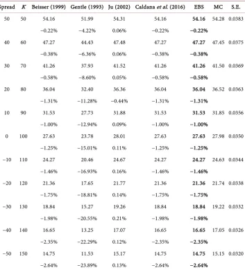
In what follows, we will show that, using the same parameter setting, our approx-imating formula is as accurate as the best methods compared in [34]. For sake of com-pleteness, we will compare it with the approaches discussed in [26], since the authors focused on the same numerical example. The results reported in Table 1 refer to the pricing of the basket option above for different strike prices K, where K varies from 50 to 150. In particular, we rounded up to two decimals the results of our calculations in order to be consistent with the precision chosen in [34]. If we compare the results of the approximating formulas in Table 1, we can see that our formula has the same level of accuracy as the one in [26], with the advantage that no optimization routine has to be run2_{. Besides that, our approximation is as accurate as the one proposed in [13]. As} pointed out in Section 1, under the geometric Brownian motion case, the second ap-proximating formula discussed in [26] coincides with the one in [15], which is less ac-curate than the other methods. We investigated the accuracy of our approximating formula by varying the input parameters as done in [34] and we found that our ap-proximating formula has the same level of accuracy as the one considered in [13]. Re-sults are available upon request.

5.1.2. Multi-Asset Spread Options

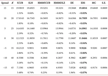
In this section we deal with the pricing of multi-asset spread options under the assump-tion of lognormality for the underlying asset prices. In particular, we compare our ap-proximating formula in Equation (26) with the four different methods discussed in [35], namely:

• _{Improved Comonotonic Upper Bound (ICUB) as in Section 2.2 in [35],}

2_{Up to the fourth decimal, our formula coincides with the one proposed in [26]. This imply that our educated}

[image:16.595.198.552.113.504.2]

959 Table 1. Prices of Basket Options (with M = 4, N = 0) computed for different strike prices K in the GBM model of Section 3. Column EBS contains the Extended Bjerksund and Stensland pric-ing formula of Section 3.

Spread K Beisser (1999) Gentle (1993) Ju (2002) Caldana et al. (2016) EBS MC S.E. 50 50 54.16 51.99 54.31 54.16 54.16 54.28 0.0383

−0.22% −4.22% 0.06% −0.22% −0.22%

40 60 47.27 44.43 47.48 47.27 47.27 47.45 0.0375 −0.38% −6.36% 0.06% −0.38% −0.38%

30 70 41.26 37.93 41.52 41.26 41.26 41.50 0.0369 −0.58% −8.60% 0.05% −0.58% −0.58%

20 80 36.04 32.40 36.36 36.04 36.04 36.52 0.0363 −1.31% −11.28% −0.44% −1.31% −1.31%

10 90 31.53 27.73 31.88 31.53 31.53 31.85 0.0356 −1.00% −12.94% 0.09% −1.00% −1.00%

0 100 27.63 23.78 28.01 27.63 27.63 27.98 0.0350 −1.25% −15.01% 0.11% −1.25% −1.25%

−10 110 24.27 20.46 24.67 24.27 24.27 24.63 0.0344 −1.46% −16.93% 0.16% −1.46% −1.46%

−20 120 21.36 17.65 21.77 21.36 21.36 21.74 0.0338 −1.75% −18.81% 0.14% −1.75% −1.75%

−30 130 18.84 15.27 19.26 18.84 18.84 19.22 0.0332 −1.98% −20.55% 0.21% −1.98% −1.98%

−40 140 16.65 13.25 17.07 16.65 16.65 17.05 0.0326 −2.35% −22.29% 0.12% −2.35% −2.35%

−50 150 14.75 11.53 15.17 14.75 14.75 15.15 0.0320 −2.64% −23.89% 0.13% −2.64% −2.64%

• _{Shifted Log-Normal Approximation (SLN) as in [9],}

• _{Hybrid Moment Matching with Improved Comonotonic Upper Bound (HMMICUB)} as in Section 3.1 in [35] and

• _{Hybrid Moment Matching with Deng et al. (2008) Spread Approximation} (HMMDLZ) as in Section 3.1 in [35].

As benchmark values, the authors in [35] consider a Monte Carlo simulation. Input parameters are as in [35], where the authors focused on spread call options written on three assets (see Table 4 and Table 7 in [35], whose weights are given by

(

)

w= 1.0, 1.0, 1.0− − ).

EK in Table 2, Table 3).

The results reported in Table 2, Table 3 refer to the pricing spread options for dif-ferent strike prices K. In particular, in Table 2, the input parameters are as follows:

1

T− =t , r=0.05, S

( )

t =

[

100, 24, 46

]

, σ =

[

0.40, 0.22, 0.30

]

, σ =

[

0.40, 0.22, 0.30

]

,

13 0.91

ρ

= _,

ρ

13=0.91. For the results in Table 3, the input parameters are as follows: 1

T− =t , T− =t 1, S

( )

t =

[

100, 63,12

]

, σ =

[

0.21, 0.34, 0.63

]

, σ =

[

0.21, 0.34, 0.63

]

,

[

0.21, 0.34, 0.63

]

σ = ,

ρ

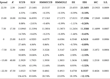
23=0.43.

In both scenarios, our approximating formula outperforms the best methods consi-dered in [35] as well as the approach in [7]. The approximation is less accurate for very deep out-of-the-money options, especially for the second case.

5.2. Non-Gaussian Models

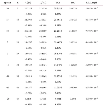
In this section we deal with the pricing of basket and multi-asset spread options where the underlying asset prices follow the stochastic dynamics reported in Sections 4. In particular, we compare our approximating formula in Equation (6) with the the two approaches discussed in [26], namely:

•

C

_K

( )

t

, as in Equation (18), • AG

( )

K

[image:17.595.193.551.456.709.2]

C

t

, based on the arithmetic-geometric average inequality, as in [26], Section 2. Input parameters are as in [26]. For all the computations involving a Fourier inver-sion, we used a Gaussian quadrature rule, using Matlab’s built-in function quadgk and a damping coefficient α =0.75 as done in [26].

Table 2. Prices of Multi-Asset Spread Options (with M = 1, N = 2) computed for different strike prices K in the GBM model of Section 3. Column EBS contains the Extended Bjerksund and Stensland pricing formula of Section 3. Number of simulations equal to 300 millions of paths and column label S.E. stands for Standard Error.

Spread K ICUB SLN HMMICUB HMMDLZ EK EBS MC S.E. 15 15 19.9819 19.6925 19.5251 19.5231 19.5848 19.6816 19.6849 0.0009

1.51% 0.04% −0.81% −0.82% −0.51% −0.02%

10 20 17.0143 16.7345 16.5693 16.5673 16.6366 16.7009 16.7051 0.0008 1.85% 0.18% −0.81% −0.82% −0.41% −0.03%

5 25 14.4105 14.1460 13.9964 13.9944 14.0731 14.0961 14.1010 0.0008 2.19% 0.32% −0.74% −0.76% −0.20% −0.03%

0 30 12.1523 11.9059 11.7811 11.7790 11.8687 11.8466 11.8519 0.0007 2.53% 0.46% −0.60% −0.62% 0.14% −0.04%

−5 35 10.2123 9.9851 9.8898 9.8876 9.9890 9.9226 9.9281 0.0007 2.86% 0.57% −0.39% −0.41% 0.61% −0.06%

−10 40 8.5588 8.3506 8.2860 8.2837 8.3962 8.2897 8.2951 0.0006 3.18% 0.67% −0.11% −0.14% 1.22% −0.07%

[image:18.595.197.552.128.383.2]

961 Table 3. Prices of Multi-Asset Spread Options (with M = 1, N = 2) computed for different strike prices K in the GBM model of Section 3. Column EBS contains the Extended Bjerksund and Stensland pricing formula of Section 3. Number of simulations equal to 15 millions of paths and column label S.E. stands for Standard Error.

Spread K ICUB SLN HMMICUB HMMDLZ EK EBS MC S.E. 22.50 2.50 24.6617 23.1681 23.5137 23.5138 23.4535 23.5493 23.5925 0.0009

4.53% −1.80% −0.33% −0.33% −0.59% −0.18%

15.00 10.00 18.5944 16.8591 17.1363 17.1373 17.0131 17.1596 17.2049 0.0008 8.08% −2.01% −0.40% −0.39% −1.11% −0.26%

7.50 17.50 13.0945 11.3394 11.3854 11.3873 11.2434 11.3588 11.4099 0.0007 14.76% −0.62% −0.21% −0.20% −1.46% −0.45%

0 25.00 8.4135 6.9203 6.6579 6.6584 6.5548 6.5418 6.6009 0.0006 27.46% 4.84% 0.86% 0.87% −0.70% −0.89%

−7.50 32.50 4.064 3.7629 3.3226 3.3147 3.2670 3.1203 3.1872 0.0004 50.80% 18.06% 4.25% 4.00% 2.50% −2.10%

−15.00 40.00 2.3929 1.7925 1.3950 1.3853 1.3636 1.1852 1.2518 0.0003 91.16% 43.19% 11.44% 10.66% 8.93% −5.32%

−22.50 47.50 1.0323 0.7369 0.4861 0.4913 0.4758 0.3537 0.4026 0.0001 156.41% 83.04% 20.74% 22.03% 18.19% −12.15%

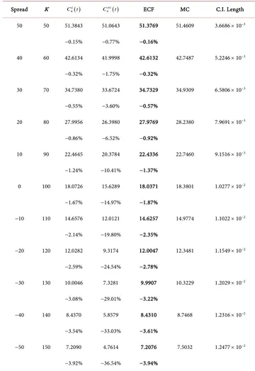
5.2.1. Basket Options

In Table 4 and Table 5, we report the results of our approximation formula when pricing basket options on 4 and 20 assets under the jump-diffusion model of Section 4.1 and the mean-reverting jump-diffusion model of Section 4.2 respectively.

As pointed out in [26], available methods in the literature which are based on the knowledge of the characteristic function, such as [29] [36][37] and [38], suffer from the curse of dimensionality, as they require an M-dimensional quadrature and therefore they cannot be used in practice when the basket dimension is high. Besides that, the first three methods require assumptions on the form of the characteristic function that rule out mean-reverting models, therefore not applicable even to the mean-reverting jump-diffusion model considered in Section 4.2.

In order to deal with the curse of dimensionality, we are aware of a method discussed in [39], where the authors propose a parallel partitioning approach. However, they do not provide results for basket options with dimension grater than seven.

[image:19.595.189.549.182.706.2]

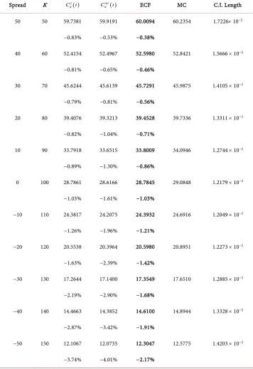
Table 4. Prices of Basket Options (with M = 20, N = 0) computed for different strikes K in the JD model of Section 4.1. The basket weights are 20

1 20 =

w 1 . The model parameters are: T− =t 1, 0.01

r= , S_k

( )

t =100, σk=0.40, k =0.5, vk =0.30, ak =mk= −0.05, λ=1, λk=0.5,

0.5 kl

ρ = _and Y 0.5 kl

ρ = for k l, =1,, 20 and k≠l, 1 otherwise. Column ECF contains the

Extended Caldana and Fusai pricing formula of Section 2. Columns MC and C.I. Length contain the Monte Carlo option price and 95% confidence interval. The Monte Carlo price is obtained with 1000000 simulations, see [26].

Spread K CK( )t

 AG( )

K

C t ECF MC C.I. Length

50 50 51.3843 51.0643 51.3769 51.4609 3.6686 × 10−3

−0.15% −0.77% −0.16%

40 60 42.6134 41.9998 42.6132 42.7487 5.2246 × 10−3

−0.32% −1.75% −0.32%

30 70 34.7380 33.6724 34.7329 34.9309 6.5806 × 10−3

−0.55% −3.60% −0.57%

20 80 27.9956 26.3980 27.9769 28.2380 7.9691 × 10−3

−0.86% −6.52% −0.92%

10 90 22.4645 20.3784 22.4336 22.7460 9.1516 × 10−3

−1.24% −10.41% −1.37%

0 100 18.0726 15.6289 18.0371 18.3801 1.0277 × 10−2

−1.67% −14.97% −1.87%

−10 110 14.6576 12.0121 14.6257 14.9774 1.1022 × 10−2

−2.14% −19.80% −2.35%

−20 120 12.0282 9.3174 12.0047 12.3481 1.1549 × 10−2

−2.59% −24.54% −2.78%

−30 130 10.0046 7.3281 9.9907 10.3229 1.2029 × 10−2

−3.08% −29.01% −3.22%

−40 140 8.4370 5.8579 8.4310 8.7468 1.2316 × 10−2

−3.54% −33.03% −3.61%

−50 150 7.2090 4.7614 7.2076 7.5032 1.2477 × 10−2

[image:20.595.197.548.186.565.2]

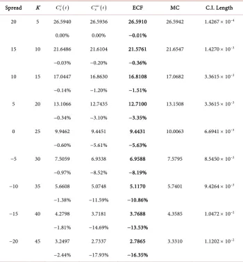
963 Table 5. Prices of Basket Options (with M = 4, N = 0) computed for different strikes K in the MRJD model of Section 4.2. The basket weights are w=

(

0.25,0.25,0.25,0.25

)

. The model pa-rameters are: T − t = 1, r = 0, fk

( )

t =ln 25

( )

, ω=

( ) (

ωk k= 0.1,0.2,0.1,0.3

)

, Y tk

( )

=Xk

( )

t =0 for k = 1, ∙∙∙, 4. Jump parameters are λ+=λ−=

(

0.1,0.2,0.3,0.2

)

and µ+=µ−=

(

0.1,0.1,0.3,0.3

)

. The covariance matrix for the Brownian part is equal to (0.5, 0.35, 0.35, 0.25, 0.35; 0.35, 0.50, 0.475, 0.15; 0.35, 0.475, 0.50, 0.15; 0.25, 0.15, 0.15, 0.50). Column ECF contains the Extended Caldana and Fusai pricing formula of Section 2. The Monte Carlo price is obtained with 100000 simulations and 100 time steps, see [26]. Columns labels are the same as in Table 4.

Spread K CK( )t

 AG( )

K

C t ECF MC C.I. Length

20 5 26.5940 26.5936 26.5910 26.5942 1.4267 × 10−4

0.00% 0.00% −0.01%

15 10 21.6486 21.6104 21.5761 21.6547 1.4270 × 10−3

−0.03% −0.20% −0.36%

10 15 17.0447 16.8630 16.8108 17.0682 3.3615 × 10−3

−0.14% −1.20% −1.51%

5 20 13.1066 12.7435 12.7100 13.1508 3.3615 × 10−3

−0.34% −3.10% −3.35%

0 25 9.9462 9.4451 9.4431 10.0063 6.6941 × 10−3

−0.60% −5.61% −5.63%

−5 30 7.5059 6.9338 6.9588 7.5795 8.5450 × 10−3

−0.97% −8.52% −8.19%

−10 35 5.6608 5.0748 5.1170 5.7401 9.4264 × 10−3

−1.38% −11.59% −10.86%

−15 40 4.2798 3.7181 3.7688 4.3585 1.0472 × 10−2

−1.81% −14.69% −13.53%

−20 45 3.2497 2.7337 2.7865 3.3310 1.1202 × 10−2

−2.44% −17.93% −16.35%

Results for the mean-reverting jump-diffusion model in Table 5 show that our ap-proximating formula is outperformed by the first approach in [26]. In this case, it seems that an optimization routine for the optimal parameters is required to produce better results. However, the accuracy of our approximating formula is still higher than the second approach in [26] and the approximation is still accurate for in-the-money options.

5.2.2. Multi-Asset Spread Options