Content-based Image Retrieval (CBIR) using Hybrid
Technique
1
Zainab Ibrahim Abood
Electrical Engineering Department, University ofBaghdad, Iraq
2
Israa Jameel Muhsin
Physics Department, Collegeof Science, University of Baghdad, Iraq
3
Nabeel Jameel Tawfiq
Remote Sensing Unit, Collegeof Science, University of Baghdad, Iraq
ABSTRACT
Image retrieval is used in searching for images from images database. In this paper, content – based image retrieval (CBIR) using four feature extraction techniques has been achieved. The four techniques are colored histogram features technique, properties features technique, gray level co-occurrence matrix (GLCM) statistical features technique and hybrid technique. The features are extracted from the data base images and query (test) images in order to find the similarity measure. The similarity-based matching is very important in CBIR, so, three types of similarity measure are used, normalized Mahalanobis distance, Euclidean distance and Manhattan distance. A comparison between them has been implemented. From the results, it is concluded that, for the database images used in this work, the CBIR using hybrid technique is better for image retrieval because it has a higher match performance (100%) for each type of similarity measure so; it is the best one for image retrieval.
Keywords
CBIR, feature extraction, properties, color histogram, GLCM, hybrid, similarity measure.
1.
INTRODUCTION
CBIR allows extracting the correct images according to objective visual contents of the image [1]. The aim of the CBIR systems is to provide means to find images in large repositories using its contents as low level descriptors. These descriptors do not exactly match the high level semantics of the image; therefore, assessing similarity between two images using only their features is not a trivial task [2].
One of the methods to index each image is a simple color histogram. It is very effective, computationally efficient and because of its low complexity, it is popular in indexing applications [1].
For face classification, two methods used to extract features using (GLCM). The first one extracts the statistical Haralick features from the GLCM in nearest neighbor and neural networks classifiers, and the second one is directly uses GLCM, which is superior to the first method [3].
Based on stationary wavelet transform combining with directional filter banks, Qingwei Gao, introduced a depeckling method for Synthetic aperture radar (SAR) images. The threshold method is substituted by Bayesian maximum a posteriori (MAP) estimation, in order to achieve more satisfying results. Stationary wavelet transform, contour-let transform and stationary wavelet combining with directional filter banks for de-speckling SAR images are used and compared [4].
The basic property of point-to-hyper plane Mahalanobis distance is exploited to recalculate bounds on query-cluster distances [5]. Chaur-Chin Chen introduced Euclidean distance
and chord distance, to test a set of six Brodatz’s textures [6]. The oldest dissimilarity measures used to compare images is Manhattan norm or sum of absolute intensity differences [7]. Retrieval of a query image from a database of images is considered as an important task in the image processing and computer vision [8].
2. FEATURE EXTRACTION:
The basic idea of CBIR is that a set of features is used, that allows to find images that are similar to the used query image. For different properties of images, different features may account [9]. The goal of the feature extraction is to find an informative variables based on image data, so, it can be seen as a kind of data reduction [10].
2.1 Color Histogram (H):
Color histogram is a statistical measure of an image. Every image has a signature associated with it and it based on its pixel values and it can be color, texture, shape, etc.
A color space is a model for representing color in terms of intensity values and it is a one- to four- dimensional space. The probability mass function of the image intensities is called an image histogram. The color histogram is defined by,
(1)
where A, B and C represent the three color channels (R, G, B) and n is the number of pixels in the image. Computationally, the color histogram is firstly performed by discretizing the colors of the image and then counting the number of pixels of each color in the image. The color histogram can be used as a set of vectors. In gray-scale image, one dimensional vector gives the value of the gray-level and the other gives the count of pixels at the gray-level, so, it has two dimensional vectors, while in color image, the color histograms are 4-D vectors [11].
2.2 Properties Features:
Some features are dependent on the properties of the image, such as mean, median and standard deviation, where:
Mean: Average or treats the columns of the image as vectors, then returning a row vector of mean values.
Mean = (2)
Median: Treats the columns of the image as vectors, then returning a row vector of median values.
(3)
where =
and n is the number of pixels in the image [8].
2.3 Gray Level Co-occurrence Matrix
(GLCM):
Some feature extraction is done by creating a gray-level co-occurrence matrix (GLCM) from each image, then extracting statistical features from each GLCM, such as, energy and contrast.
Energy: it is the sum of squared elements in the GLCM:
(4)
where (i, j) is correspond to the number of occurrences of the gray level’s pair, when i and j are the gray levels [13]. Contrast: it is indicates the variance of the gray level [14].
(5)
2.4 Wavelet transform:
In this work two types of wavelet transform are used,
discrete wavelet transform and stationary wavelet transform:
2.4.1 Discrete Wavelet Transform (DWT):
By using DWT, an image can be decomposed into a different spatial resolution image. In case of a 2D image, if N level decomposition is performed, then the result is 3N+1 different frequency bands as shown in Fig. (1)[15]. In a multilevel wavelet filter bank, iterating the lowpass and highpass filter, then a down-sampling procedure only on the previous stage’s low-pass branch output [16].
Fig.1: 2D- Discrete Wavelet Transform [15]
2.4.2 Stationary Wavelet Transform (SWT):
The Discrete Wavelet Transform is not a time-invariant transform [15].Nason and Silverman are proposed a stationary wavelet transform (SWT), which is shift invariant and redundant, it is also called un-decimated wavelet transform. To image stationary wavelet transform, the 2-D image x(n, n) ,(where n×n is the size of the image) is transformed into four subbands which can be labeled as LL, LH, HL and HH as shown in Fig. (2).
The LL subband comes from low pass filtering and it is most like the original image. The remaining subbands LH, HL and HH are called detailed components. The LH contains horizontal details, HL contains the vertical details;, while HH contains the diagonal details only [4].
Fig.2: 2D - Stationary Wavelet Transform [4]
3. SIMILARITY MEASURE:
A measurement of how close a vector to another vector is called similarity measurement [6].The query image features are used to retrieve the similar images from the image database. Instead of directly comparing two images, similarity of the query image features is measured with the features of each image in the database. Computing the distance between the feature vectors is the measure of similarity between two images. The retrieval systems return the first images, whose distance from the query image is minimum [8].The distance measurements such as, Mahalanobis distance; Euclidean distance, Manhattan distance and Histogram intersection distance (HID) are indicated in this work. Mahalanobis distance: it is the distance between a query and database images feature vectors. Let q be the feature vector for the query image and y is the feature vector for the database image to be compared, so, the Mahalanobis distance between q and y is calculated as:
Mahal diatance = (6)
where is the inverted covariance matrix [9].
Euclidean distance: is a distance measured between two feature vectors q and y:
(7)
Manhattan distance: is a distance measured between two feature vectors q and y [8]:
(8) CAj Rows Rows CAj+1 CDj+1 CDj+1 Horizontal CDj+1 Columns Columns Vertical Diagonal Columns Columns Lo_D
Hi_D
1 ↓ 2 1 ↓ 2
Lo_D
Hi_D
Lo_D
Hi_D
2 ↓ 1 2 ↓ 1 2 ↓ 1 2 ↓ 1 1 ↓ 2 2 ↓ 1
Where Down sample column: keep the even indexed columns Down sample row: keep the even indexed rows
Histogram Intersection Distance (HID): for color image retrieval, the intersection of color histograms h and g is given by:
d (h, g ) = (9)
where |h| and |g| are the magnitude of each histogram. Colors which are not present in the query image do not contribute to the intersection distance. [11].
4. THE PROPOSED TECHNIQUE
ALGORITHM:
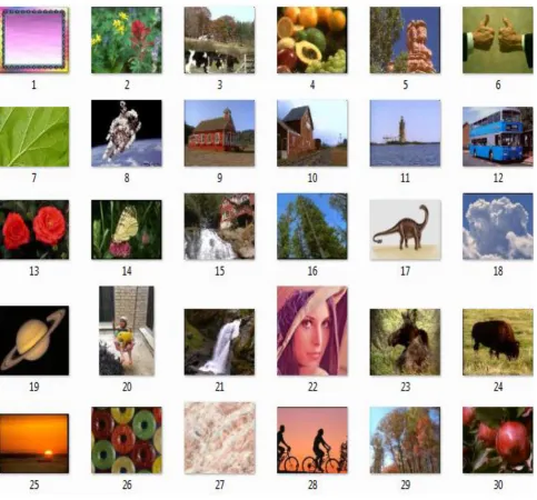
The proposed technique is a CBIR using four feature extraction techniques, (309) image as a database and (39) image as query image, the proposed algorithm is as follows: 1. Input the color image; take the three color channels R, G and B independently on each other.
2. In other side, convert the color image to a gray scale. 3. Resize R, G, B and gray image into a square image of size (n×n) where n=128 pixels.
4. Histogram features are extracted from each R, G, B color and gray images of the query and database images as a histogram features technique.
5. Features dependent on the properties of the image are extracted from each R, G, B color and gray images of the query and database images as a properties features technique using equations (2) and (3) respectively.
6. For each gray image, create a gray-level co-occurrence matrix (GLCM) from each image in query and database and extracting statistical features from each GLCM of query and database images as a GLCM statistical features technique using (4) and (5) respectively.
7. For each gray image, apply a single-level stationary wavelet transform (SWT) (db5) then apply a second level of
DWT (haar) to the Low- Low sub-band of SWT, finally, apply the third level of DWT (haar) to the Low-Low sub-band of the DWT. The Low-Low sub-band of the third level is considered as a feature for image retrieval, so, it is created for each image in query and database as a hybrid wavelet features technique.
8. For each technique, in steps 4, 5, 6 and 7, construct vectors for the features of each image in data base and each image in query images, so, the number of vectors is equal to the number of images in the data base and query images. 9. By using equations 6, 7, 8 and 9, the similarity was measured between the features vectors of query and database images for each technique.
5. TESTING AND EVALUATION OF
THE RESULTS:
There are four figures showing the results for the proposed system when applied on one of the test image as a model, also there are four tables showing the results measured for the proposed system:
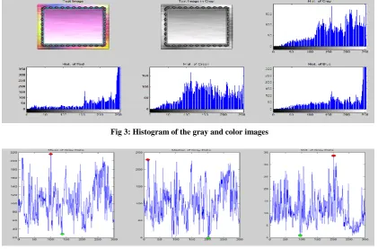
Figure (3) shows a sub plot of the color image, gray image and its histogram and and R, G, B channel’s histograms. Figure (4) shows a sub plot of the mean, median and standard deviation of gray image. The red dot refers to maximum value and the green dot refers to minimum value.
Figure (5) shows a subplot oft Euclidean and Manhattan distance for mean, median and standard deviation. The red dot refers to maximum distance value and the green dot refers to minimum distance value and that the test image is match with the image number 32 in database.
[image:3.595.86.508.455.732.2]Figure (6) shows the histogram Mahalanobis; Euclidean, Manhattan and intersection distance. The red dot refers to maximum distance value and the green dot refers to minimum value of distance and that the test image is match with the image number 32 in database.
Fig 3: Histogram of the gray and color images
Fig 5: Mean, median, standard deviationof the Euclidian and Manhattan distance
Fig 6: Histogram of the Mahalanobis, Euclidian, Manhattan, and intersection distance
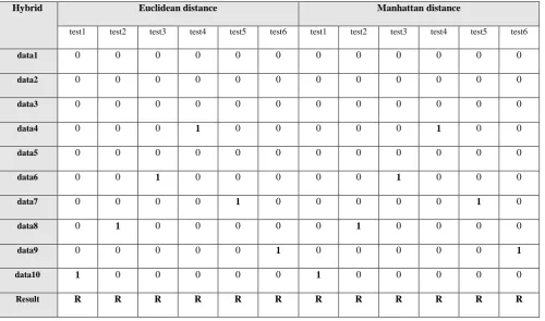
The first three tables, 1, 2 and 3 showing the results measured for the proposed system when applied on the database and query images in case of that the database included some images that are the copy of the test images. While, tables 4, 5 and 6 show the results in case that the database not included any copy of the test image, but included some images nearly similar to that in the test images.
Table1 shows the similarity measure for the histogram and properties features. Histogram, mean and standard deviation have maximum average value so, they are good for image retrieval and the images are 100% retrieved for Mahalanobis, Euclidean, Manhattan and Histogram intersection distance. Table2 shows the similarity measure for the GLCM, Number “1” refers to “Retrieved” and number “0” refers to “Not retrieved”. In Mahalanobis distance, test 1, 4 and 6 are not retrieved, while in Euclidean, Manhattan distance all test images are retrieved so, they are good for image retrieval,
where, R: Recognized and NR: Not Recognized.
Table 3 shows the similarity measure for the hybrid features. All test images are retrieved so, it is good for image retrieval. Table 4 shows the similarity measure for the histogram and properties features. In Euclidean, Manhattan and Histogram intersection distance using histogram features, it can be seen that the rate of matching is 55% or more, while the mean, median and standard deviation have zero matching value so, they are not suitable for image retrieval using Euclidean and Manhattan distance.
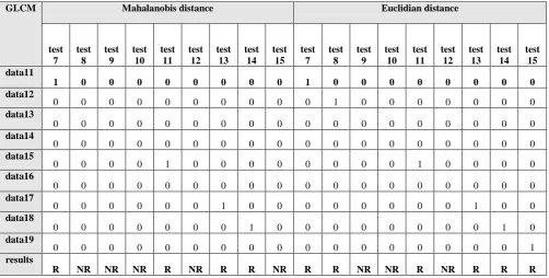
Table 5a and table 5b shows the similarity measure for the GLCM, for all types of distance, some of test images are retrieved and some of them are not retrieved so; they are not suitable for image retrieval.
[image:4.595.53.545.627.752.2]Table 6 shows the similarity measure for the hybrid features, for all types of distance, all test images are retrieved so, it is the best technique for image retrieval.
Table 1. Similarity measure for the histogram and properties features
Features test image (1-30)
Histogram Mean Median Std.
Mahal. Eclud. Manh. HID Eclud. Manh. Eclud. Manh. Eclud. Manh.
Rate of matching
Table 2. Similarity measure for GLCM features
GLCM
Mahalanobis distance Euclidean distance Manhattan distance
test1 test2 test3 test4 test5 test6 test1 test2 test3 test4 test5 test6 test1 test2 test3 test4 test5 test6
data1 0 0 0 0 0 0 0 0 0 0 0 0 0 0 0 0 0 0
data2 0 0 0 0 0 0 0 0 0 0 0 0 0 0 0 0 0 0
data3 0 0 0 0 0 0 0 0 0 0 0 0 0 0 0 0 0 0
data4 0 0 0 0 0 0 0 0 0 1 0 0 0 0 0 1 0 0
data5 0 0 0 0 0 0 0 0 0 0 0 0 0 0 0 0 0 0
data6 0 0 1 0 0 0 0 0 1 0 0 0 0 0 1 0 0 0
data7 0 0 0 0 1 0 0 0 0 0 1 0 0 0 0 0 1 0
data8 0 1 0 0 0 0 0 1 0 0 0 0 0 1 0 0 0 0
data9 0 0 0 0 0 0 0 0 0 0 0 1 0 0 0 0 0 1
data10 0 0 0 0 0 0 1 0 0 0 0 0 1 0 0 0 0 0
Results NR R R NR R NR R R R R R R R R R R R R
Table 3. Similarity measure for hybrid features
Hybrid Euclidean distance Manhattan distance
test1 test2 test3 test4 test5 test6 test1 test2 test3 test4 test5 test6
data1 0 0 0 0 0 0 0 0 0 0 0 0
data2 0 0 0 0 0 0 0 0 0 0 0 0
data3 0 0 0 0 0 0 0 0 0 0 0 0
data4 0 0 0 1 0 0 0 0 0 1 0 0
data5 0 0 0 0 0 0 0 0 0 0 0 0
data6 0 0 1 0 0 0 0 0 1 0 0 0
data7 0 0 0 0 1 0 0 0 0 0 1 0
data8 0 1 0 0 0 0 0 1 0 0 0 0
data9 0 0 0 0 0 1 0 0 0 0 0 1
data10 1 0 0 0 0 0 1 0 0 0 0 0
[image:5.595.51.552.444.739.2]Table 4. Similarity measure for the histogram and properties features
Features test image (31-39)
Histogram Mean Median Std.
Mahal. Eclud. Manh. HID Eclud. Manh. Eclud. Manh. Eclud. Manh.
Rate of matching
0% 55% 55% 66% 0% 0% 0% 0% 0% 0%
Table 5a. Similarity measure for the GLCM features using Manhattan distance
GLCM Manhattan distance
test7
test8
test9
test10
test11
test12
test13
test14
test15
data11
1
0
0
0
0
0
0
0
0
data12
0
1
0
0
0
0
0
0
0
data13
0
0
0
0
0
0
0
0
0
data14
0
0
0
0
0
0
0
0
0
data15
0
0
0
0
1
0
0
0
0
data16
0
0
0
0
0
0
0
0
0
data17
0
0
0
0
0
0
1
0
0
data18
0
0
0
0
0
0
0
1
0
data19
0
0
0
0
0
0
0
0
0
Results
R
R
NR
NR
R
NR
R
R
NR
Table 5b. Similarity measure for the GLCM features using mahalanobis and Eclusian distance
GLCM Mahalanobis distance Euclidian distance
test 7
test 8
test 9
test 10
test 11
test 12
test 13
test 14
test 15
test 7
test 8
test 9
test 10
test 11
test 12
test 13
test 14
test 15 data11
1 0 0 0 0 0 0 0 0 1 0 0 0 0 0 0 0 0
data12
0 0 0 0 0 0 0 0 0 0 1 0 0 0 0 0 0 0
data13
0 0 0 0 0 0 0 0 0 0 0 0 0 0 0 0 0 0
data14
0 0 0 0 0 0 0 0 0 0 0 0 0 0 0 0 0 0
data15
0 0 0 0 1 0 0 0 0 0 0 0 0 1 0 0 0 0
data16
0 0 0 0 0 0 0 0 0 0 0 0 0 0 0 0 0 0
data17
0 0 0 0 0 0 1 0 0 0 0 0 0 0 0 1 0 0
data18
0 0 0 0 0 0 0 1 0 0 0 0 0 0 0 0 1 0
data19
0 0 0 0 0 0 0 0 0 0 0 0 0 0 0 0 0 1
results
[image:6.595.49.552.452.706.2]Table 6: Similarity measure for the hybrid features
6. CONCLUSIONS:
As a conclusion, CBIR using the proposed technique Hybrid technique has a higher match performance (i.e., 100%) in all types of similarity measure and in each two cases, the database included some images that are the copy of the test images or not included, so it is the best technique. When using the case of that the database included images the same as that in the test images (only in this case), histogram, mean and standard deviation have maximum rate of matching 100%, so, they are good for image retrieval for Mahalanobis, Euclidean, Manhattan and Histogram intersection distance.
7. REFERENCES:
[1] S. Selvarajah and S. R. Kodithuwakku “Combined Feature Descriptor for Content Based Image Retrieval”, 2011 6th International Conferencon Industrial and Information Systems, ICIIS 2011, Aug. 16-19, 2011, Sri Lanka, IEEE.
[2] M. Arevalillo-Herr´aez, Francesc J. Ferri, Salvador Moreno-Picot, “An interactive evolutionary approach for content based image retrieval”, Proceedings of the 2009 IEEE International Conference on Systems, Man, and Cybernetics San Antonio, TX, USA - October 2009, www.ivsl.org .
[3] A. Eleyan, Hasan Demirel, “Co-occurrence Matrix and its Statistical Features as a New Approach for Face Recognition”, Turk J Elec. Eng. & Comp. Sci., Vol.19, No.1, 2011, www.ivsl.org.
[4] Qingwei Gao, Yanfei Zhao, Yixiang Lu, “Despeckling SAR images using stationary wavelet transform combining with directional filter banks”, 2008, [email protected]
[5] S.Ramaswamy and Kenneth Rose, “Fast Adaptive Mahalanobis Distance - Based Search and Retrieval in Image Databases”, 2008,www.ivsl.org .
[6] C. Chin Chen ∗and H. Ting Chu, “Similarity Measurement between Images”, 2005, [email protected]
[7] A. A. Goshtasby, Image Registration, “Similarity and Dissimilarity Measures”, 2012, ch2.
[8] T. Acharya , Ajoy K. Ray, “Image Processing Principles and Applications”, Book, 2005, Published by John Wiley & Sons, Inc., Hoboken, New Jersey.
[9] T. Deselaers, “Features for Image Retrieval”, 2003. [10] M. Egmont - Petersen, D. de Ridder, H. Handels,”Image
Processing with Neural Networks—a review”, 2002. [11] R. Dubey, R. Choubey, S. Dubey, “Efficient Image
Mining using Multi Feature Content Based Image Retrieval System”, IntJr of Advanced Computer Engineering and Architecture, Vol. 1, No. 1, June 2011, [email protected],
[12] Math Works, Inc., “Image Processing Toolbox”, Matlab 7.8.0 (R2009a)”, 2009.
[13] B. Wang, Hang-jun Wang, Heng-nian Qi, ”Wood Recognition Based on Grey-Level Co-Occurrence Matrix”, International Conference on Computer
Hybrid Euclidian distance Manhattan distance
test 7
test 8
test 9
test 10
test 11
test 12
test 13
test 14
test 15
test 7
test 8
test 9
test 10
test 11
test 12
test 13
test 14
test 15
data11 1
0 0 0 0 0 0 0 0 1 0 0 0 0 0 0 0 0
data12 0 1 0 0 0 0 0 0 0 0 1 0 0 0 0 0 0 0
data13 0
0 1 0 0 0 0 0 0 0 0 1 0 0 0 0 0 0
data14 0
0 0 1 0 0 0 0 0 0 0 0 1 0 0 0 0 0
data15 0
0 0 0 1 0 0 0 0 0 0 0 0 1 0 0 0 0
data16 0
0 0 0 0 1 0 0 0 0 0 0 0 0 1 0 0 0
data17 0
0 0 0 0 0 1 0 0 0 0 0 0 0 0 1 0 0
data18 0 0 0 0 0 0 0 1 0 0 0 0 0 0 0 0 1 0
data19 0 0 0 0 0 0 0 0 1 0 0 0 0 0 0 0 0 1
Application and System Modeling (ICCASM 2010), IEEE, www.ivsl.org.
[14] H.B.Kekre, Sudeep D. Thepade, Tanuja K. Sarode and Vashali Suryawanshi, “Image Retrieval using Texture Features extracted from GLCM, LBG and KPE”, International Journal of Computer Theory and Engineering, Vol. 2, No. 5, October, 2010,www.ivsl.org [15] Kanagaraj Kannan, Subramonian Arumuga Perumal,
Kandasamy Arulmozhi, “Optimal Decomposition Level
of Discrete, Stationary and Dual Tree Complex Wavelet Transform for Pixel based Fusion of Multi-focused Images”, Serbian Journal of Electrical Engineering, Vol. 7, No. 1, May 2010, 81-93, Email- [email protected] , [email protected] , [email protected].
[image:8.595.56.540.211.661.2][16] Michael B. Martin and Amy E. Bell, “New Image Compression Techniques Using Multiwavelets and Multiwavelet Packets”, IEEE Transactions on Image Processing, Vol. 10, No. 4, April 2001.