Optimal Asset Allocation Strategy for Defined Contribution Pension Plans with Different Power Utility Functions

How to cite this paper: Ma, Q.P. (2014) Optimal Asset Allocation Strategy for Defined-Contribution Pension Plans with Dif- ferent Power Utility Functions. Open Access Library Journal, 1: e754. http://dx.doi.org/10.4236/oalib.1100754

Optimal Asset Allocation Strategy for

Defined-Contribution Pension Plans with

Different Power Utility Functions

Qingping Ma

Department of Quantitative and Applied Economics, Nottingham University Business School (China), The University of Nottingham Ningbo China, Ningbo, China

Email: [email protected]

Received 12 April 2014; revised 22 May 2014; accepted 2 July 2014

Copyright © 2014 by author and OALib.

This work is licensed under the Creative Commons Attribution International License (CC BY).

http://creativecommons.org/licenses/by/4.0/

Abstract

The relationship between the optimal asset allocation and the functional form of power utility is investigated for defined-contribution (DC) pension plans. The horizon dependence of optimal pension portfolios is determined by the argument of the power utility function. The optimal com- position of pension portfolios is horizon independent when terminal utility is a power function of wealth-to-wage ratio, and deterministically horizon dependent when terminal utility is a function of terminal wealth or replacement ratio (the pension-to-final wage ratio). The optimal portfolios all contain a speculative component to satisfy the risk appetite of DC plan members, which is do- minated by bonds under usual market assumptions. The optimal compositions of financial wealth on hand (the sum of pension portfolio and the short-sold wage replicating portfolio) are stochas- tically horizon dependent when wages are fully hedgeable and stochastic. The optimal pension portfolios also have a preference free component to hedge wage risk, when terminal utility is a function of wealth-to-wage ratio or replacement ratio. A state variable dependent component in optimal pension portfolios exists when terminal utility is a function of terminal wealth or replace- ment ratio, but it disappears when terminal utility is a function of terminal wealth-to-wage ratio and the risk premium is constant.

Keywords

Defined-Contribution Pension Plan, Wage Risk, Optimal Asset Allocation, Power Utility, Hamilton-Jacobi-Bellman Equation

Subject Areas: Business Finance and Investment, Insurance, Risk Management

1. Introduction

OALibJ | DOI:10.4236/oalib.1100754 2 July 2014 | Volume 1 | e754

form of consumption and portfolio problem. Most studies on the consumption and portfolio allocation strategies over multiple periods are built upon the classical dynamic optimization model by Merton [1], which assumes a constant interest rate and constant risk premium without wage income. Since empirical studies show that sto- chastic variations in interest rates and in risk premiums exist, it may not be appropriate to assume a constant in- terest rate for portfolios with a long horizon such as pension funds. Later studies extend Merton’s work with stochastic interest rates [2]-[4] or stochastic risk premiums [5]. Since contribution from wage income is also important for pension wealth growth, studies on DC plan strategies generally assume stochastic interest rates and deterministic or stochastic wages [6]-[10].

With stochastic interest rates, the financial market is usually assumed to have three types of asset: cash, bonds and equities (stocks). Boulier et al. [7], Deelstra et al. [8] and Battocchio and Menoncin [9] use these three as- sets in their studies on optimal asset allocation strategies for DC pension plans. In those studies, the stock price follows a geometric Brownian motion which includes volatilities from risk sources of both the interest rate and the stock market. Although stochastic interest rates make bonds distinct from cash and equities, in some studies bonds are not explicitly differentiated from other risky assets. Vigna and Haberman [6] assume two assets: one low risk asset and one high risk asset. Cairns et al. [10] use one risk-free asset and N risky assets, and the return on each risky asset follows a geometric Brownian motion with volatilities of N risk sources.

One important difference between pension fund asset allocation problem and Merton’s consumption and portfolio problem is that, the objective of pension plans is to maximize the terminal utility and there is no con- sumption or consumption-derived utility before retirement. The optimal allocation strategy for a DC pension plan depends critically on the specifications of terminal utility function. Boulier et al. [7] and Deelstra et al. [8]

assume that terminal utility is a power function of cash lump sum over a guaranteed minimum benefit; Battoc- chio and Menoncin [9] assume an exponential function of real wealth (wealth-to-price index ratio). To relate terminal utility with the existing standard of living, Cairns et al. [10] assume that terminal utility is a function of wealth-to-wage ratio or replacement ratio (pension-to-final wage ratio). The use of replacement ratio is more appropriate for an individual who intends to convert her pension wealth into a life annuity on retirement, which suggests that she is more risk averse and perceiving life annuities as good value.

Using one risk-free asset and N risky assets and assuming that terminal utility is a power function of terminal wealth-to-wage ratio or replacement ratio, Cairns et al. [10] find that optimal asset allocation in risky assets needs three efficient mutual funds if the terminal utility is a function of replacement ratio. One mutual fund (which is heavily dominated by equities) is to satisfy the risk appetite of the plan member. The second fund (which is heavily dominated by cash) is to hedge the wage risk. The third fund (which is heavily dominated by bonds) is to hedge interest rate risk. Cairns et al. [10] call the three funds “equity”, “cash” and “bond” funds re- spectively. If the terminal utility is a function of wealth-to-wage ratio, the optimal asset allocation needs only the “equity” fund and the “cash” fund.

Although Cairns et al. [10] indicated that the “equity”, “cash” and “bond” funds are heavily dominated by equi- ties, cash and bonds respectively; they did not provide a measure on how to gauge the dominance. Is it possible that the “equity” fund is dominated by bonds in some scenarios? The present paper tries to answer this question and extends the study of Cairns et al. [10] by investigating the composition of those mutual funds. For simplicity, I assume that the pension plan can invest in three assets, cash, bond and stock [7]-[9], and investigate three dif- ferent scenarios: the terminal utility is a function of terminal wealth, a function of terminal wealth-to-wage ratio or a function of replacement ratio. The assumption of wealth-to-wage ratio or wealth as the argument of terminal utility function is more appropriate for individuals who are reluctant to annuitize their pension wealth on retirement. This paper is organized as follows. Section 2 formulates the financial market, wage and pension wealth growth models. Section 3 presents the optimization problem and the Hamilton-Jacobi-Bellman equation. Section 4 solves the optimal asset allocation problem for power utility when pension contribution has stopped or wage risk is fully hedgeable. Section 5 discusses and summarizes the results in this paper.

2. The Model

2.1. Market Structure

OALibJ | DOI:10.4236/oalib.1100754 3 July 2014 | Volume 1 | e754

ty asset, a stock, available, which can be considered as the index of a stock market. The uncertainty in the finan- cial market is described by two standard and independent Brownian motions Zr(t) and ZS(t) with t∈

[ ]

0,T , de-

fined on a complete probability space (Ω, F, P) where P is the real world probability. The filtration F = F(t)

[ ]

0,

t T

∀ ∈ generated by the Brownian motions can be interpreted as the information set available to the inves- tor at time t.

The instantaneous risk-free rate of interest r(t) follows an Ornstein-Uhlenbeck process (Vasicek model)

( )

(

( )

)

( )

( )

0

dr t =α β−r t dt+σ_rdZ_r t , r 0 =r. (1) In Equation (1), α and β are strictly positive constants, and σr is the volatility of interest rate. The stochastic

element Zr(t) causes the process to fluctuate in an erratic, but continuous fashion [11].

When the interest rate process is described by Equation (1), the price of zero-coupon bonds for any date of maturity τ at time t, B(t, τ, r), is governed by the diffusion equation [7] [8] [11]

(

)

(

)

(

( ) ( )

)

( )

( )

( )

d , ,

, d , d , , 1,

, , r r r

B t r

r t b t t b t Z t B

B t r

τ

τ σ ξ τ σ τ τ

τ = + − =

where ξ is the market price of interest rate risk assumed to be constant, and

( )

1 e ( ) ,

t

b t

α τ

τ

α

− −

−

= .

The riskless asset has a price process governed by

( )

( ) ( )

( )

0

dR t =R t r t d ,t R 0 =R. (2) The riskless asset can be considered as a cash fund paying the instantaneous interest rate r(t) without any de- fault risk. The value of the cash fund at t is then

( )

( )

0 exp ₀t

( )

d R t =R _ r s s_



∫

. (3) There are zero-coupon bonds for any date of maturity, and a bond rolling over zero coupon bonds with con- stant maturity K. The price of the zero coupon bond with constant maturity K is denoted by BK(t, r) with

( )

( )

( )

( )

d ,

d d

, K

K r K r r

K

B t r

r t b t b Z t

B t r = + σ ξ − σ , (4)

where

1 e K K

b

α

α

−

−

= .

The relationship between B(t, τ, r) and BK(t, r) through the riskless cash asset R(t) [7] is

(

)

(

)

( )

( )

( )

( )

( )

( )

d , , , d , d ,

1

, , ,

K

K K K

B t r b t R t b t B t r

B t r b R t b B t r

τ τ τ

τ

 

= −  +

  .

The above equation shows that the “rolling bond” can be obtained by a portfolio of one zero coupon bond and the cash asset, and that other bonds can also be obtained through a portfolio of the riskless asset and the “rolling bond”.

The stock has a process of the total return governed by stochastic differential equation (SDE)

( )

( )

( )

( )

( )

( )

0

dS t =S t _µ_S r t, dt+v_rSσ_rdZ_r t +σ_SdZ_S t _, S 0 =S , (5) where

( )

,

( )

S r t r t mS

µ = + (6) is the instantaneous percentage change in stock price per unit time. The volatility scaling factor vrS measures

OALibJ | DOI:10.4236/oalib.1100754 4 July 2014 | Volume 1 | e754

2.2. Wages

The plan member’s wage, Y(t), evolves according to the SDE

( )

( )

(

( ) ( )

)

( )

( )

( )

( )

0

dY t =Y t _ µ_Y t +r t dt+v_rYσ_rdZ_r t +v_SYσ_SdZ_S t +σ_YdZ_Y t _, Y 0 =Y , (7) where μY(t) is a deterministic function of time, age and other individual characteristics such as education and

occupation. These assumptions on wage processes are similar to those by Battocchio and Menoncin [9] and Cairns et al. [10]. Here σY is a constant and ZY(t) a standard Brownian motion, independent of Zr(t) and ZS(t).

The volatility scaling factors, vrY and vSY, measure how interest rate volatility and stock volatility affect wage vo-

latility, respectively. The parameter σY is a non-hedgeable volatility whose risk source does not belong to the set

of the financial market risk sources. When σY = 0, the market is complete. Otherwise the market is incomplete.

3. The Optimization Problem and Hamilton-Jacobi-Bellman Equation

3.1. Terminal Utility Is a Function of Terminal Wealth

The value of the plan member’s pension wealth at time t is denoted by W(t), and the proportions of fund wealth invested in the riskless asset, bonds and stock are denoted as θR(t), θB(t) and θS(t) respectively,

( )

( )

( )

1

R t B t S t

θ +θ +θ = , (8) The SDE governing the pension wealth process is

( )

( ) (

)

( )

( ) (

)

(

)

( )

{

}

( )(

)

( )

(

1

) ( )

( )

1

( )

1

d d d

d 1 d

1 d

d d

d d .

B S B S

B S B K r S S

B K S rS r r S S S

R B S

W t W t Y t t

R B S

W t r r b Y t t

W t b v Z W t Z

M r W t Y t t W t Z

θ θ θ θ π

θ θ θ σ ξ θ µ π

θ θ σ θ σ

θ π θ

 

= _ − − + + _+

 

 

= _ − − + + + _+

+ − + +

′ ′

=_ + + _ + Γ

(9)

where π is the proportion of wage contributed to the pension plan and Y(t) is the wage income at period t,

[

]

1

[

]

1 1

[

]

0

, , k r , .

B S K r S r S

rS r S

b

M B m Z Z Z

v

σ

θ

θ

θ

σ ξ

σ

σ

−

 

′

′≡ ≡ Γ ≡′ _{ } ′≡

  (10)

The stochastic optimal control problem can be written as follows:

( )

(

)

maxE U W T ,T

θ  ,

subject to

(

)

( )

( )

1 1

1 1

0 0

d d d ,

0 , 0 , 0 ,

w

w

t Z

M r W Y W

W

w w W W t T

µ

θ π θ

′ Ω

   

 _{= +}

   

  _{′ + + ′ ′Γ}

     

= = ∀ ≤ ≤

(11)

where

[

]

w≡ r Y ′, µ_w ≡_α β

(

−r

)

Y

(

µ_Y +r

)

_′, 1

0 r

rY r SY S

Yv Yv

σ

σ

σ

 

′

Ω ≡  

 

The solution to this problem should give us the optimal portfolio composition. The Hamiltonian correspond- ing to the optimization problem (11) is

( )

(

)

2 2 2 2

1 1 1 2 1 1 1 1 2

1 1

.

2 2

t w

J J J J J

H J J M r W Y tr W W

w W w w W W

µ′ ∂ θ′ π ∂  ′ ∂  θ′ ′ ∂ θ′ ′ θ ∂

= + +_ + + _ + _Ω Ω _+ Γ Ω + Γ Γ

∂ ∂ _ ∂ _ ∂ ∂ ∂ (12)

OALibJ | DOI:10.4236/oalib.1100754 5 July 2014 | Volume 1 | e754

2 2

2

1 1 1 1 1 2 0

H J J J

M W W W

W w W θ W

θ

∂ ₌ ∂ _{+ Γ Ω′} ∂ _{+ Γ Γ′} ∂ ₌

∂ ∂ ∂ ∂ ∂ , (13)

where H

θ

∂

∂ is a vector. The optimal portfolio composition is

(

)

1

(

)

1 *

1 1 1 1 1 1 1

W wW

WW WW

J J

M

WJ WJ

θ

_′ − _′ − _′

= − Γ Γ − Γ Γ Γ Ω . (14)

Here *

( )

*

( )

*

B t S t

θ _{= }θ θ ′

 , the optimal proportions invested in bonds and stock respectively. The two terms on the right hand side of Equation (14) can be designated as θ₁∗ and θ₂∗ respectively, which are them- selves vectors with two elements corresponding to certain proportions of investment in bonds and stock. We can summarize the above results as

Proposition 1: If the terminal utility is a power function of terminal wealth, the optimal composition in risky assets has two components, the speculative component

(

_{1 1}

)

1 ₁ W

WW

J M

WJ

−

′

− Γ Γ (fund 1) to satisfy the risk appetite

of the plan members and the component

(

1 1

)

1 1 1 wW

WW

J WJ

−

′ ′

− Γ Γ Γ Ω (fund 2) to hedge financial market risk.

3.2. Terminal Utility Is a Function of Terminal Wealth-to-Wage Ratio

Applying Itô’s lemma, we get the SDE governing the wealth-to-wage ratio X t

( )

=W t

( ) ( )

Y t ,

( )

( )

2

(

)

2 3 2

1 1

dX t dW W dY W dY d dW Y

Y Y Y Y

= − + − . (15)

By substituting the value of W, Y, dW and dY, the SDE governing this pension wealth-to-wage ratio process is:

( ) (

)

(

)

dX t =_θ′M+u X+π_dt+ θ′ ′Γ + Λ′ X Zd , (16) where,

[

]

[

]

2

2 2 2 2 2

2 2

2

2

, ,

0 0

, ,

0

.

K r K rY r

Y rY r SY S Y

S rY rS r SY S

K r

rY r SY S Y

rS r S

r S Y

b b v

M u v v

m v v v

b

v v

v

Z Z Z Z

σ ξ σ _{µ σ σ σ}

σ σ

σ

σ σ σ

σ σ

 + 

≡_{ } ≡ − + + +

− −

 

−

 

′ ′

Γ ≡_{ } Λ ≡ − − −

 

′ ≡

(17)

The optimal asset allocation problem is to find the strategy θ that maximizes the expected terminal utility of a plan member,

( )

(

)

maxE U X T ,T

θ  ,

subject to

(

)

(

)

d w w dt dZ

M u X X

X

µ

θ π θ

′ Ω

   

 

=_{ } +_{ }

  _{′ + + ′ ′Γ + Λ}

      (18)

where,

0 0

r

rY r SY S Y

Yv Yv Y

σ

σ

σ

σ

 

′

Ω ≡  

 . (19)

OALibJ | DOI:10.4236/oalib.1100754 6 July 2014 | Volume 1 | e754

( )

(

)

(

)

(

)

2

2

2 2

2 2

1 2

1

2 .

2

t w

J J J

H J J M u x tr

w X w

J J

x x

w X X

µ θ π

θ θ θ θ

 

∂ ∂ ∂

′ ′ ′

= + _∂ +_ + + _∂ + Ω Ω 

∂

 

∂ ∂

′ ′ ′ ′ ′ ′ ′ ′

+ Γ + Λ Ω + Γ Γ + Γ Λ + Λ Λ

∂ ∂ ∂

(20)

Differentiating Equation (20) with respect to θ gives the first-order condition

(

)

2 2

2

2 0

H J J J

Mx x x

X w X θ X

θ

∂ ₌ ∂ _{+ Γ Ω′} ∂ _{+ Γ Γ + Γ Λ′ ′} ∂ ₌

∂ ∂ ∂ ∂ ∂ , (21)

The optimal portfolio composition is

( )

1

( )

1

( )

1

* X wX

XX XX

J J

M

xJ xJ

θ _′ − _{′ ′} − _′ − _′

= − Γ Γ Γ Λ − Γ Γ − Γ Γ Γ Ω . (22)

The three terms on the right hand side of Equation (22) can be designated as θ₀∗, θ₁∗ and θ₂∗ respectively, and the additional term θ₀∗ compared with Equation (14) is a preference-free hedging component to hedge wage risk. The three terms on the right-hand-side of Equation (22) correspond to the optimal asset allocation strategy with three mutual funds labeled as “cash”, “bond” and “equity” in Cairns et al. [10].

3.3. Terminal Utility Is a Function of Replacement Ratio

Applying Ito’s formula to current replacement ratio

( )

( )

( )

(

,

( )

( )

)

P t X t G t

Y t a t r t

= = where P(t) is the pension in-

come if annuitizing the pension wealth now and a t r t

(

,

( )

)

the annuity rate, gives the SDE governing the re- placement ratio

( )

_{( )}

( )

( )

( )

( )

( )

( )

2

2 3 2

1 1

d d d , d , d d ,

, , , ,

X X

G t X a t r a t r X a t r

a t r a t r a t r a t r

= − + _ _ − _ _. (23)

The process governing a t r t

(

,

( )

)

uses the expression by Cairns et al. [10],

( ) ( )

1

( )

2

( ) (

)

( )

d , , d d

2 a r a a r r

a t r =a t r __ c r

σ

−d r

α β

−r _ t−d r

σ

Z _

 

  (24)

In the above equation, d_a

( )

r is the duration of the annuity function, c r_a

( )

is its convexity

( )

_{( )}

1

( )

, ,

a

a t r

d r

a t r r

∂ = −

∂ ,

( )

( )

( )

2

2

, 1

, a

a t r c r

a t r r ∂ =

∂ . (25)

By substituting W, dW, X, a t r t

(

,

( )

)

, dX and da t r

( )

, , the SDE governing the replacement ratio process is:

( )

2 2

(

2

)

dG t M G u G dt G Zd

a

π

θ θ

 _′  _{′ ′ ′}

=_ + + _ + Γ + Λ

  , (26)

where

(

)

(

)

(

)

(

)

[

]

2

2 2 2

2 2 2 2 2

2

2

,

1

, 2

0 0

, , .

0

K r rY a K r

S rY a rS r SY S

Y rY a rY a a r SY S Y a

K r

a rY r SY S Y r S Y

rS r S

b v d b

M

m v d v v

u v d v c d v d r

b

d v v Z Z Z Z

v

σ ξ σ

σ σ

µ σ σ σ α β

σ

σ σ σ

σ σ

 + − 

=  _{− − −} 

 

 

 

= − +_ − − + _ + + + −

 

−

  _{′ ′}

′  

Γ =_{ } Λ =_ − − − _ =

 

(27)

OALibJ | DOI:10.4236/oalib.1100754 7 July 2014 | Volume 1 | e754

( )

(

)

maxE U G T ,T

θ  ,

subject to

(

2 2

)

(

2

)

d d d

w

w

t Z

G

G M u G

a

µ

π _θ

θ

  _{ Ω′ }

  ₌  _{+  }

   ′ + +  ′ ′Γ + Λ

  _{ }   . (28)

The Hamiltonian is similar to the wealth-to-wage ratio case and the optimal portfolio composition is

( )

1

( )

1

( )

1 *

2 2

G wG

GG GG

J J

M

GJ GJ

θ _′ − _{′ ′} − _′ − _′

= − Γ Γ Γ Λ − Γ Γ − Γ Γ Γ Ω . (29)

We can summarize the results in subsections 3.2 and 3.3 as

Proposition 2: If the terminal utility is a power function of wealth-to-wage ratio or replacement ratio, the op- timal portfolio for DC pension plans in risky assets consists of three funds: 1) a preference-free hedging com- ponent to hedge wage risk, 2) a speculative component to satisfy the risk appetite of the plan members, and 3) a state variable dependent hedging component to cover the plan member from financial market risk.

4. Optimal Asset Allocation Strategy for Power Terminal Utility

Since when there is non-hedgeable wage risk, the optimal portfolio problem for power utility has no analytical solution, the present study will only look at the scenario where wages can be fully hedged. When wage income is fully hedgeable

(

σ =Y 0

)

, let Q be the risk-neutral pricing measure and Z tr

( )

and ZS

( )

t independent

standard Q-Brownian motions [10], the wage process under Q is

( )

( )

(

( ) ( )

)

( )

( )

dY t =Y t _ µ_Y t +r t −ξ_{r rY}v σ_r−ξ_Sv_SYσ_S dt+v_rYσ_rdZ_r t +v_SYσ_SdZ_S t _, (30) which implies that

( )

( )

( ) ( )

(

)

( )

( )

( )

( )

}

2 2 2 2

1 1

exp d

2 2

.

Y r rY r S SY S rY r SY S

t

rY r r r SY S S S

Y Y t s r s s v v v v t

v Z Z t v Z Z t

τ

τ µ ξ σ ξ σ σ σ τ

σ τ σ τ

  

= _ _ + _ −_ + + + _ −

 



   

+ _ − _+ _ − _

∫

   

(31)

Here ξr is a measure of how interest/bond volatility will affect wage, and ξS is a scale factor measuring how

stock price volatility affects wages. The market value at time t for future contributions to the pension plan paya- ble between t and T is then

( )

{

}

( )

( )

( )

(

)

( )

( )

( )

( )

}

( )

{

( )

(

)(

)

}

( ) ( )

2 2 2 2

exp d d

1 1

exp d

2 2

d

exp d d

. T

Q _{t t} t

T

Q _{t t} Y r rY r S SY S rY r SY S

rY r r r SY S S S t

T

Y r rY r S SY S

t t

E r s s Y F

E Y t s s v v v v t

v Z Z t v Z Z t F

Y t s s v v t

Y t f t

τ

τ

τ

π τ τ

π µ ξ σ ξ σ σ σ τ

σ τ σ τ τ

π µ ξ σ ξ σ τ τ

π

 ₋ 

 

 

   

= _{ } −_ + + + _ −

 

 



   

+ _ − _+ _ − _{ }

= − + −

=

∫

∫

∫

∫

∫

∫

    (32)

OALibJ | DOI:10.4236/oalib.1100754 8 July 2014 | Volume 1 | e754

composition of the replicating portfolio can be written in vector form

1

rS SY rY R

K B

R R

S SY

R

R rS SY rY

SY

K v v v

b v v v v v

b

θ

θ θ

θ

−

 

 

 _{  }

 _{  }

=_{  }=



  _{ − }

  _{− −}

 

 

. (33)

In the above equation, the superscript R indicates replicating portfolio.

4.1. Terminal Utility Is a Power Function of Terminal Wealth

Since future contributions have been added to enhance the current pension wealth, the Hamiltonian Equation (12) becomes

( )

(

1

)

1 1 22

2 2

2

1 1 1 1 2

1

2

1

. 2

t w

J J J

H J J M r W tr

w W w

J J

W W

w W W

µ θ

θ θ θ

 

∂ ∂ ∂

′ ′ ′

= + + + + _Ω Ω _

∂ ∂ _ ∂ _

∂ ∂

′ ′ ′ ′

+ Γ Ω + Γ Γ

∂ ∂ ∂

(34)

I start with a trial solution by assuming that the value function has the form

(

)

1

( )

1

(

)

, , , , , 1 .

1

J t W w g t wγW γ g T w w

γ

−

= = ∀

− (35)

Substituting the partial derivatives of the value function and the optimal proportion composition of pension fund investment θ*

, Equation (14), and simplifying (see Appendix A for detailed derivation), the Equation (12) becomes

(

)

(

)

( )

(

)

1 1

1 1 1 1 1 1 1 2 1 1 1 1

1 1 1 1

0.

2 ₂

t w w ww

g

µ

γ

M g tr g

γ

M M

γ

r g

γ

γ

γ

−  − 

 _′ − _{′ ′ ′}  _′ − _{′ ′} −

+_ + Γ Γ Γ Ω _ + Ω Ω − Γ Γ −  =

−

 

  _{ } (36)

By the Feynman-Kac formula [12][13], there exists a probability measure Q(γ) such that

( )

(

,

)

Q( )

(

,

( )

)

( )

, t

g t w t =E _γ _g T w T D t T F_, (37) where w s

( )

is governed by the SDE

( )

(

( )

)

(

( )

)

dw s =µ _w w s ds+ Ω w s ,s ′dZ, µ_w

(

w s

( )

)

µ_w 1 γ M₁

(

_{1 1}

)

1 ₁

γ

−

− _{′ ′ ′}

= + Γ Γ Γ Ω

  , w t

( )

=w t

( )

, and

( )

, exp T

( )

d t

D t T = _ ϕ s s_ 

∫

,

where

( )

( )

(

)

1 1 1 1 1 2

1 1

2

s

γ

M M

γ

r

ϕ

γ

γ

−

 _{− −} 

′ ′

= − Γ Γ − 

−

 

 

.

In Equation (37), Ft is the filtration, which can be interpreted as the information available to the investor at

time t. The optimal composition is

(

)

1

(

)

1

( )

*

1 1 1 1 1 1 1

1

d T

t t

t

M E s s

w

θ ϕ

γ

− − ∂

′ ′ ′

= Γ Γ + Γ Γ Γ Ω _ _

∂

∫

,

OALibJ | DOI:10.4236/oalib.1100754 9 July 2014 | Volume 1 | e754

are zero,

(

)

1

(

)

1

[ ]

*

1 1 1 1 1 1 1

1 1 d T t t t

M E r s

w γ θ γ γ − − − ∂ ′ ′ ′

= Γ Γ + Γ Γ Γ Ω

∂

∫

. (38)

The first term of the optimal composition in the above equation is

(

)

1 2 2

₍

2

₎

1 1 1 1 2 2

1 1

.

rS r S rS S r

K r S K rS r S r

v v m

M

b b v m

σ ξ σ ξ

σ

θ

γ

γ σ σ

σ ξ

σ

−

∗_{= Γ Γ′ =} _ + + _

+

 

 

The second term (see Appendix B for detailed derivation)

(

)

1

[ ]

( )

2 1 1 1

1 1 e 1

d . 0 t T T t t t K

E r s

w b α γ γ θ γ αγ − −

∗₌ − _{Γ Γ′ Γ Ω′} ∂ ₌ −  − 

 

∂ _{ }

∫

This state variable dependent hedging component contains only bonds and it is horizon-dependent. The op- timal proportions of pension wealth invested in bonds and equities are

(

)

( )

2 2 2 2

2 2

1 1 e 1

. 0 t T

rS r S rS S r

B

K

K r S

S K rS r S r

v v m

b

b b v m

α

σ ξ σ ξ

σ

θ

γ

αγ

γ σ σ

θ

σ ξ

σ

∗ − ∗  + +     _{=  +} − −     ₊  

  _{ }   (39)

When the terminal utility is a function of terminal wealth, the optimal composition of financial wealth is

( ) ( )

( )

( ) ( )

( )

( ) ( )

( )

( )

( ) ( )

( )

2 2 2 2

2

2

1

1 e 1

1

0

F R

B B B

F R

S S S

rS r S rS S r

t T K r S

K rS r S

S

rS SY rY

K

SY

Y t f t Y t f t

W t W t

v v m

Y t f t b

W t v m b

v v v Y t f t

b W t

v

α

π π

θ θ θ

θ θ θ

σ ξ σ ξ σ

π γ σ σ γ

αγ σ ξ γσ π ∗ ∗ −         = +  −   _{ }            + +       _{  −}  ₋ _ = +_ _{  }+  _ + _{ }  _{  } _{ }    −   − _  .     _ (40)

In the above equations, θ_BF and θ_SF are the optimal proportions of financial wealth invested in bonds and stocks respectively, and θ_BR and θ_SR are proportions of the replicating portfolio short-sold in bonds and stocks respectively. The optimal proportion of the financial wealth invested in risk-free assets is

( )

F 1

( )

F

( )

F

R t B t S t

θ = −θ −θ .

4.2. Terminal Utility Is a Power Function of Wealth-to-Wage Ratio

When the terminal utility is a power function of wealth-to-wage ratio, Equation (20) becomes

( )

(

)

(

)

(

)

2 2 2 2 2 2 1 2 1 2 . 2 t w

J J J

H J J M u x tr

w X w

J J

x x

w X X

µ θ

θ θ θ θ

 

∂ ∂ ∂

′ ′ ′

= + + + + _Ω Ω _

∂ ∂ _ ∂ _

∂ ∂

′ ′ ′ ′ ′ ′ ′ ′

+ Γ + Λ Ω + Γ Γ + Γ Λ + Λ Λ

∂ ∂ ∂

(41)

Substituting the partial derivatives of the value function

(

)

1

( )

1

, , ,

1

J t x w g t wγ x γ

γ

−

=

OALibJ | DOI:10.4236/oalib.1100754 10 July 2014 | Volume 1 | e754

(

)

(

)

( )

(

)

(

)

1 1 1 2 1 1 2

1 1 1

0. 2

t w w ww

g M g tr g

M M M u g

γ µ

γ

γ γ γ

γ γ

γ

−

− −

 _′ − _{′ ′ ′}  _′

+_ + Γ Γ Γ Ω_ + Ω Ω

 

 _{− − −} 

′ ′ ′ ′ ′

− Γ Γ + Γ Γ Γ Λ −  =

−

 

 

(42)

Using Feynman-Kac formula, the optimal portfolio composition is

( )

1

( )

1

( )

1

( )

* 1 d T t t t

M E s s

w

θ ϕ

γ

− − − ∂

′ ′ ′ ′ ′

= − Γ Γ Γ Λ − Γ Γ + Γ Γ Γ Ω _ _

−

∫

∂ , (43)

where

( )

( )

( )

( )

1 1

2

1 1 1

2

s

γ

M M

γ

M

γ

u

ϕ

γ

γ

γ

− −  _{− − −}  ′ ′ ′ ′ ′

= − Γ Γ + Γ Γ Γ Λ − 

−

 

 

.

Since all the terms in the function φ(s) do not depend on the state variables r and Y, its derivatives with re- spect to wt are zero and the above equation becomes

(

)

1

(

)

1

* _M 1

θ

γ

− −

′ ′ ′

= − Γ Γ Γ Λ + Γ Γ . (44)

The first term in the above equation is

(

)

1 2 2 2 2

0 2 2 2 2 2 2

1 K rY r S K rS SY r S 1 rS SY rY

K SY K

K r S K SY r S

v v v

b v b v v

b v b

b b v

σ σ σ σ

θ

σ σ σ σ

−

∗ _{= − Γ Γ′ Γ Λ =′} −  − ₌  − 

 ₋   

 

  ;

The second term is

( )

1 2 2 2

₍

2

₎

2

1 2 2 2

1 1

.

rS r S rY r S rS S r rS SY r S

K r S K rS r S r SY r S

v v v m v v

M

b b v m v

σ ξ σ ξ

σ σ

σ

σ σ

θ

γ

γ σ σ

σ ξ

σ

σ σ

−

∗ _{= Γ Γ′ =} _ + + + − _

+ −

 

 

The optimal proportions of pension wealth invested in bonds and equities are

(

)

2 2 2 2 2

2 2 2

1 1

.

rS r S rY r S rS S r rS SY r S

rS SY rY B

K SY

K K r S

S K rS r S r SY r S

v v v m v v

v v v

b v

b b b v m v

σ ξ σ ξ

σ σ

σ

σ σ

θ

γ σ σ

θ

σ ξ

σ

σ σ

∗ ∗  + + + −  −     _{ } = +     _{ + − }  

  _{ } (45)

The optimal proportion of pension wealth invested in risk-free assets is

1

R B S

θ∗_{= −}θ∗₋θ∗_.

The optimal composition of financial wealth is

( ) ( )

( )

( ) ( )

( )

( ) ( )

( )

2 2 2 2 2

2 2 2 1 1 F R

B B B

F R

S S S

rS r S rY r S rS S r rS SY r S rS SY rY

K r S K

rS r S SY S SY

S Y t f t Y t f t

W t W t

v v v m v v

v v v

b Y t f t

b

W t v m v

v

π π

θ θ θ

θ θ θ

σ ξ σ ξ σ σ σ σ σ

γ σ σ π

σ ξ σ

γσ ∗ ∗         = +  −   _{ }            + + + −  −   _{ }      =_{  }+ + _{  } + −             (46)

4.3. Terminal Utility Is a Power Function of Replacement Ratio

When the terminal utility is a power function of replacement ratio, substituting the partial derivatives of the val-

ue function

(

)

1

( )

1

, , ,

1

J t G w g t wγG γ

γ

−

=

− and the optimal proportion composition of pension fund investment θ*

[image:11.595.157.538.334.444.2]

OALibJ | DOI:10.4236/oalib.1100754 11 July 2014 | Volume 1 | e754

( )

(

)

( )

( )

1 2

1 1

2 2 2 2 2 2

1 1

2

1 1 1

0. 2( )

t w w ww

g M g tr g

u M M M g

γ µ

γ

γ γ γ

γ γ γ

−

− −

 _′ − _{′ ′ ′}  _′

+_ + Γ Γ Γ Ω_ + Ω Ω

 

 − − _{′ ′ ′} − _′ 

+_ − Γ Γ Γ Λ − Γ Γ _ =

−

 

(47)

Using the Feynman-Kac formula, the optimal pension portfolio composition is

( )

1

( )

1

( )

1

( )

*

2 2 ₂

1

d T

t t

t

M E s s

w

θ ϕ

γ

− − − ∂

′ ′ ′ ′ ′

= − Γ Γ Γ Λ + Γ Γ − Γ Γ Γ Ω _ _ ∂

∫

, (48)

where

( )

( )

( )

( )

1 1

2 2 2 2 2 2

1 1 1

2

s γ u γ M γ M M

ϕ

γ γ γ

− −

− − _{′ ′ ′} − _{′ ′}

= − Γ Γ Γ Λ − Γ Γ

− .

Since only u2 explicitly depends on the state variables,

( )

1

( )

1

( )

1

[ ]

*

2 2 2 2

1 1

d T

t t

t

M E u s

w

γ θ

γ γ

− − − − ∂

′ ′ ′ ′ ′

= − Γ Γ Γ Λ + Γ Γ + Γ Γ Γ Ω ∂

∫

. (49)

It is necessary to find out the modified process of r for computing integral in the third term in Equation (49) in the same way as in Section 4.1 when terminal utility is a power function of terminal wealth. The optimal propor- tions of pension wealth invested in bonds and equities are

(

)

(

)

( )

(

)

2 2 2 2 2

2 2 2 2

1

1

e 1

1

. 0

a rY rS SY

B

K SY K

S

rS r S rY a r S rS S r rS SY r S

K r S K rS r S r SY r S

t T a K

d v v v

b v b

v v d v m v v

b b v m v

d b

α

θ

θ

σ ξ σ ξ

σ σ

σ

σ σ

γ σ σ

σ ξ

σ

σ σ

γ

γ

∗

∗

−

− +

   

=

   

 

 

 + + − + − 

 

+

+ −

 

 

_{− −} 

−  

+

 

 

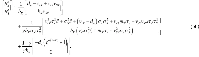
(50)

The optimal composition of the financial wealth in hand is similarly the sum of

( ) ( )

( )

1 Y t f t

W t

π

+ pension

portfolio of Equation (50) and

( ) ( )

( )

Y t f t W t

π

− wage replicating portfolio of Equation (33). From the results in Section 4, we have the following

Proposition 3: The optimal composition of DC pension portfolio with power utility functions are either static or deterministic lifestyle, the stochastic life styling in terms of pension plan financial wealth results from the stochastic wages.

The state variables dependent hedging component corresponds to the “bond” fund in Cairns et al. [10] and they conclude that “bond” fund becomes zero when the pension plan is funding for a cash lump sum. As shown in the present study, it is when funding for wealth-to-wage ratio “bond” fund becomes zero, whereas when fund- ing for a cash lump sum “bond” fund does not become zero.

Cairns et al. [10] conclude that the “equity” fund is dominated by equities, but they have not proved it be- cause they do not separate equities from bonds explicitly. In the present study, bonds and equities are explicitly separated; the “equity” term of Equations (39), (45) and (50) contains a substantial investment in bonds. To in- vestigate which asset is more dominant in the “equity” fund, the proportions of bonds and equities in the “equity” fund are calculated for different values of relative risk aversion with the parameters inTable 1, which are com- monly assumed in pension and finance studies [7]-[10]. The numerical results indicate that the speculative component or “equity” fund is actually dominated by bonds for all the three functional forms of power utility (Figure 1).

[image:12.595.141.486.97.357.2]

OALibJ | DOI:10.4236/oalib.1100754 12 July 2014 | Volume 1 | e754

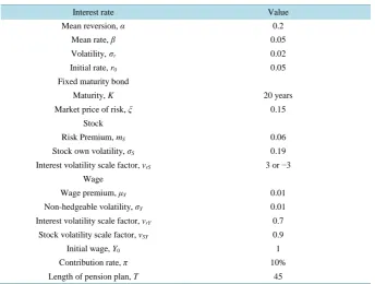
Table 1. Parameters used in numerical simulation.

Interest rate Value

Mean reversion, α 0.2

Mean rate, β 0.05

Volatility,σr 0.02

Initial rate, r0 0.05

Fixed maturity bond

Maturity, K 20 years

Market price of risk, ξ 0.15

Stock

Risk Premium, mS 0.06

Stock own volatility, σS 0.19

Interest volatility scale factor, vrS 3 or −3

Wage

Wage premium, μY 0.01

Non-hedgeable volatility, σY 0.01

Interest volatility scale factor, vrY 0.7

Stock volatility scale factor, vSY 0.9

Initial wage, Y0 1

Contribution rate, π 10%

Length of pension plan, T 45

Figure 1. The relationship between relative risk aversion coefficient γ and the optimal proportions of bond and stock in “equity fund” for pension portfolio when terminal utility is a function of wealth, wealth-to-wage ratio or replacement ratio respectively. The asset ratio range is cut off at −3 and 3 in order to show details of asset proportions when γ<1. Results for tnterest volatility scaling factor for stock vrS=3 are shown, and the results are similar for vrS≥1. (A) Terminal utility is a power function of terminal wealth; (B) Terminal utility is a power function of wealth-to-wage ratio; (C) Terminal utility is a power function of replacement ratio.

-3 -2 -1 0 1 2 3

0 1 2 3 4 5 6 7 8 9 10

A

s

se

t R

a

ti

o

Relative Risk Aversion

Cash, Bond and Stock Proportions in "Equity Fund" for Function of Wealth

Cash Bond Stock

A

-3 -2 -1 0 1 2 3

0 1 2 3 4 5 6 7 8 9 10

A

s

se

t R

a

ti

o

Relative Risk Aversion

Cash, Bond and Stock Proportions in "Equity Fund" for Function of Wealth-to-Wage Ratio

Cash Bond Stock

B

-3 -2 -1 0 1 2 3

0 1 2 3 4 5 6 7 8 9 10

A

s

se

t R

a

ti

o

Relative Risk Aversion

Cash, Bond and Stock Proportions in "Equity Fund" for Function of Replacement Ratio

Cash Bond Stock

OALibJ | DOI:10.4236/oalib.1100754 13 July 2014 | Volume 1 | e754

is shown in Figure 2(A)for the wealth-to-wage ratio case, also calculated with parameters in Table 1. It is easy to see from Figure 2(A)that an individual will stop short-selling cash for buying stock only when her relative risk aversion is high.

The absolute value of the replicating portfolio decreases as t increases (i.e. the retirement date approaches), whereas W(t) is generally increasing in t. Because the optimal composition of the augmented pension wealth is different from the composition of the replicating portfolio, the change in their relative sizes will affect the op- timal composition of their sum, the financial wealth. Therefore, although neither the optimal composition of augmented pension wealth nor the composition of the replicating portfolio is horizon dependent when the ter- minal utility is a function of terminal wealth-to-wage ratio, the optimal composition of the pension plan financial wealth is horizon-dependent. When the terminal utility is a function of lump cash sum or replacement ratio, the horizon dependence comes from both the pension portfolio per se and the change in the relative sizes between the pension portfolio and the wage replicating portfolio.

As illustrated in Figure 2(B) where parameters in Table 1and γ = 2 are used in the numerical simulation, the optimal proportions of the three assets are horizon dependent. The values of cash, bond and stock in the finan- cial wealth and the total value of financial wealth (in terms of wealth-to-wage ratio) over the life of the pension plan are shown in Figure 2(C).

The short-sold replicating portfolio is being paid off over time, so that the proportion of riskless asset in the financial wealth increases and the proportions of risky assets decrease. The optimal portfolio composition in terms of financial wealth is therefore stochastic lifestyling [10]. This is consistent with the results of Bodie et al.

[14] and Campbell and Viceira [3] that the presence of (risky) labor incomes tilts the portfolios towards risky financial assets.

Figure 2. (A) The relationship between the optimal composition of pension portfolio and the relative risk aversion coefficient when terminal utility is a power function of wealth-to-wage ratio; (B) The horizon-depen- dent profile of optimal proportions of cash, bond and stock in financial wealth for power utility over the life of the pension plan; (C) The values of cash, bond and stock in the financial wealth and the total value of financial wealth (in terms of wealth-to-wage ratio) over the life of the pension plan. For the simulation results shown in

Figure 2(B) andFigure 2(C), parameters in Table 1 are used, the relative risk aversion coefficient γ = 2 and interest volatility scaling factor for stock vrS=3. The results are from 1000 simulations.

-3 -2 -1 0 1 2 3

0 1 2 3 4 5 6 7 8 9 10

A

s

se

t R

a

ti

o

Relative Risk Aversion

Cash, Bond and Stock Proportions in Pension Wealth for Power Utility, vrs=3

Cash Bond Stock

A

-20 -15 -10 -5 0 5 10 15 20

0 10 20 30 40

A

s

se

t R

a

ti

o

Time

Optimal Proportions of Cash, Bond and Stock in Financial Wealth, γ=2

Cash Bond Stock

B

-150 -100 -50 0 50 100 150

0 10 20 30 40

W

ea

lt

h

-to

-w

a

g

e

r

a

ti

o

Time

Financial Wealth and Its Cash, Bond and Stock Components for Power Utility, γ=2

Cash Bond Stock Financial wealth

C

OALibJ | DOI:10.4236/oalib.1100754 14 July 2014 | Volume 1 | e754

5. Conclusions

In this paper the optimal portfolio problem under stochastic interest rate and wage income is solved for different functional forms of power utility, when there are three assets, cash, bonds and stock, in the financial market. Under the present model assumptions, the optimal portfolio (for an unspecified utility function) invests in both riskless and risky assets. The investment in risky assets contains three components when terminal utility is a power function of replacement ratio: a preference free hedging component, a speculative component, and a state variable dependent component. This result is consistent with that of Cairns et al. [10]. The three components are roughly corresponding to the “cash”, “equity” and “bond” funds in Cairns et al. [10]. When terminal utility is a power function of terminal wealth-to-wage ratio, the state variable dependent component disappears; when ter- minal utility is a power function of terminal wealth, the preference-free component disappears.

Closed form solution is derived for power terminal utility when there is no non-hedgeable wage risk. The state-variable dependent hedging component disappears when the expected terminal utility is a power function of wealth-to-wage ratio. The preference free hedging component and the speculative component contain both bonds and stocks, and even the speculative component (“equity” fund) can have a larger proportion of bonds, which is different from the conclusion of Cairns et al. [10]. Since both the preference free hedging component and the speculative component are horizon independent, the optimal pension asset allocation strategy of pension wealth per se is horizon independent. The positive correlation between stock returns and wage growth increases the optimal proportion invested in stocks. When the future contributions from wage incomes are hedged by short-selling a replicating portfolio, the optimal portfolio composition of pension plan financial wealth (aug- mented pension wealth + short-sold wage replicating portfolio) is horizon dependent.

To summarize, the optimal pension portfolio for the DC pension plans is horizon independent when terminal utility is a power function of pension wealth-to-wage ratio, and horizon dependent when terminal utility is a power function of terminal wealth or replacement ratio. The optimal portfolio composition of pension plan fi- nancial wealth is horizon dependent. The speculative component to satisfy the risk appetite of the plan members consists of both bonds and stocks.

Acknowledgements

The author is grateful to Prof. D. Blake, Dr. S. Wright and Dr. B. Baxter for their helpful comments and con- structive suggestions.

References

[1] Merton, R.C. (1969) Lifetime Portfolio Selection under Uncertainty: The Continuous-Time Case. Review of Economics and Statistics, 51, 247-57. http://dx.doi.org/10.2307/1926560

[2] Sørensen, C. (1999) Dynamic Allocation and Fixed Income Management. Journal of Financial and Quantitative Ana- lysis, 34, 513-532. http://dx.doi.org/10.2307/2676232

[3] Campbell, J.Y. and Viceira, L.M. (2002) Strategic Asset Allocation: Portfolio Choice for Long-Term Investors. Oxford University Press, Oxford.

[4] Liu, J. (2007) Portfolio Selection in Stochastic Environments. Review of Financial Studies, 20, 1-39.

http://dx.doi.org/10.1093/rfs/hhl001

[5] Kim, T.S. and Omberg, E. (1996) Dynamic Nonmyopic Portfolio Behavior. Review of Financial Studies, 9, 141-161.

http://dx.doi.org/10.1093/rfs/9.1.141

[6] Vigna, E. and Haberman, S. (2001) Optimal Investment Strategy for Defined Contribution Pension Schemes. Insur- ance: Mathematics and Economics, 28, 233-262. http://dx.doi.org/10.1016/S0167-6687(00)00077-9

[7] Boulier, J.F., Huang, S.J. andTaillard, G. (2001) Optimal Management under Stochastic Interest Rates: The Case of a Protected Defined Contribution Pension Fund. Insurance: Mathematics and Economics, 28, 173-189.

http://dx.doi.org/10.1016/S0167-6687(00)00073-1

[8] Deelstra, G., Grasselli, M. and Koehl, P.F. (2003) Optimal Investment Strategies in the Presence of a Minimum Guar- antee. Insurance: Mathematics and Economics, 33, 189-207. http://dx.doi.org/10.1016/S0167-6687(03)00153-7

[9] Battocchio, P. and Menoncin, F. (2004) Optimal Pension Management in a Stochastic Framework. Insurance: Mathe- matics and Economics, 34, 79-95. http://dx.doi.org/10.1016/j.insmatheco.2003.11.001

OALibJ | DOI:10.4236/oalib.1100754 15 July 2014 | Volume 1 | e754

http://dx.doi.org/10.1016/j.jedc.2005.03.009

[11] Vasicek, O.E. (1977) An Equilibrium Characterization of the Term Structure. Journal of Financial Economics, 5, 177- 188. http://dx.doi.org/10.1016/0304-405X(77)90016-2

[12] Øksendal, B. (2000) Stochastic Differential Equation—An Introduction with Applications. 5th Edition, Springer, Ber- lin.

[13] Duffie, D. (2001) Dynamic Asset Pricing Theory. 3rd Edition, Princeton University Press, Princeton and Oxford.