Development of Interest in Science and Interest in Teaching Elementary Science: Influence of Informal, School, and Inquiry Methods Course Experiences

5-4-2007

Empirical Likelihood Confidence Intervals for the Sensitivity of a

Empirical Likelihood Confidence Intervals for the Sensitivity of a

Continuous-Scale Diagnostic Test

Continuous-Scale Diagnostic Test

Angela Elaine Davis

Follow this and additional works at: https://scholarworks.gsu.edu/math_theses

Part of the Mathematics Commons

Recommended Citation Recommended Citation

Davis, Angela Elaine, "Empirical Likelihood Confidence Intervals for the Sensitivity of a Continuous-Scale Diagnostic Test." Thesis, Georgia State University, 2007.

https://scholarworks.gsu.edu/math_theses/30

This Thesis is brought to you for free and open access by the Department of Mathematics and Statistics at ScholarWorks @ Georgia State University. It has been accepted for inclusion in Mathematics Theses by an authorized administrator of ScholarWorks @ Georgia State University. For more information, please contact

Under the Direction of Gengsheng Qin

ABSTRACT

Diagnostic testing is essential to distinguish non-diseased individuals from

diseased individuals. More accurate tests lead to improved treatment and thus reduce

medical mistakes. The sensitivity and specificity are two important measurements for the

diagnostic accuracy of a diagnostic test. When the test results are continuous, it is of

interest to construct a confidence interval for the sensitivity at a fixed level of specificity

for the test. In this thesis, we propose three empirical likelihood intervals for the

sensitivity. Simulation studies are conducted to compare the empirical likelihood based

confidence intervals with the existing normal approximation based confidence interval.

Our studies show that the new intervals had better coverage probability than the normal

approximation based interval in most simulation settings.

by

ANGELA E. DAVIS

A Thesis Submitted in Partial Fulfillment of the requirements for the Degree of

Master of Science

in the College of Arts and Sciences

Georgia State University

by

ANGELA E. DAVIS

Major Professor: Dr. Gengsheng (Jeff) Qin Committee: Dr. Yu-Sheng Hsu

Dr. Yichuan Zhao Dr. Xu Zhang

Electronic Version Approved:

“To whom much is given, much more is also required.

”

ACKNOWLEDGEMENTS

I would like to thank my advisor, Dr. Gengsheng Qin, for his leadership and

patience throughout this process. Words can not express how truly grateful I am for all of

your guidance. I would also like to thank the committee members for accepting my

invitation and your assistance.

Many thanks to my parents who set the bar for my sisters and I to follow. Thank

you for all of your support as I traversed through this marvelous world of academia. I

would also like to thank my sisters for their continued support and I want you to know

that I am proud of you. Two down, one to go!

To my classmate, Kenita, from the bottom of my heart you are greatly

appreciated. Thanks for the endless encouragement. Friends come a dime a dozen but

TABLE OF CONTENTS

Acknowledgements v

List of Figures vii

List of Tables viii

Chapter I Introduction 1

Chapter II Concepts and Terminology 4

2.1 Sensitivity and Specificity of a Binary Diagnostic Test 4 2.2 Sensitivity and Specificity of a Continuous-Scale Diagnostic Test 5

Chapter III Existing Methods 6

3.1 Normal Approximation Based Confidence Interval 6

3.2 Empirical Likelihood Interval 7

Chapter IV New Confidence Intervals 9

Chapter V Simulation Studies for the Confidence Intervals 14

Chapter VI Real Application 17

6.1 Detection of Diabetes 17

Chapter VII Discussion 19

References 20

Appendix I: Simulation Tables 22

A. Normal Distribution Tables 22

B. Beta Distribution Tables 28

C. Exponential Distribution Tables 34

Appendix II: Real Application Table 40

Appendix III: S-plus Code for Simulation 41

LIST OF FIGURES

LIST OF TABLES

Chapter V Simulation studies for the confidence intervals 14

Table I. Parameter Settings for the Normal Distribution 14 Table II. Parameter Setting for the Beta Distribution 15 Table III. Parameter Settings for the Exponential Distribution 16

Appendix I Simulation Tables 22

A. Normal Distribution Tables 22

TABLE IV 22

TABLE V 23

TABLE VI 24

TABLE VII 25

TABLE VIII 26

TABLE IX 27

B. Beta Distribution Tables 28

TABLE X 28

TABLE XI 29

TABLE XII 30

TABLE XIII 31

TABLE XIV 32

TABLE XV 33

C. Exponential Distribution Tables 34

TABLE XVI 34

TABLE XVII 35

TABLE XVIII 36

TABLE XIX 37

TABLE XX 38

TABLE XXI 39

Chapter I

INTRODUCTION

Diagnostic testing, an integral facet of medical testing, aids in classifying the

presence or absence of a disease or condition. There are two types of diagnostic tests:

qualitative and quantitative. A qualitative test classifies patients as diseased or

non-diseased based on clinical signs or symptoms. A quantitative test classifies patients

according to c, a predetermined cutoff point. Disease or non-disease status is dependent

upon whether or not the test result falls above or below the cutoff point. A more accurate

diagnostic test leads to more effective treatment and thus reduces medical malpractice

and mortality. The results of a diagnostic test help to answer two questions: If the test is

positive, what is the probability that the person actually has the disease, and if the test is

negative, what is the probability that the person actually doesn’t have the disease? These

questions can simply be answered in terms of the test’s sensitivity and specificity

respectively. A model test would have high sensitivity and high specificity.

The Receiver Operating Characteristic (ROC) curve, developed in World War II,

was initially used in signal detection theory. It has since become widely used in

diagnostic medicine as an efficient way to graphically display the tradeoff between

sensitivity and specificity. When the specificity is high, the sensitivity is low and vice

versa. More specifically, a ROC curve is a plot of 1 - specificity against sensitivity. In

must be defined when the response is continuous. When a level of specificity is chosen

(commonly 80 %, 90% or 95%), it is of interest to construct confidence intervals for the

sensitivity at the selected level of specificity.

Empirical likelihood (EL), introduced by Owen (1988, 1990), is a powerful

non-parametric method. The EL method has many advantages over normal approximation

based methods. For example, it has better small sample performance than approaches

based on normal approximation; EL-based confidence regions are range preserving and

transformation respecting; the regularity conditions for EL-based methods are weak and

natural etc. The use of EL methods has becoming increasingly common in recent years

and is attractive in many applied area (Wu and Rao, 2006). Claeskens et al. (2003), one

of few studies on the EL method for ROC analysis, developed an empirical likelihood

confidence interval for a ROC curve. Their EL confidence interval had better coverage

probability than the normal approximation based interval. However, their method still

needs kernel distribution estimation and the selection of smoothing parameters are

problematic. It thus has not been well applied in practice.

In this thesis, we propose new empirical likelihood based confidence intervals and

compare them with the existing normal approximation based interval. The thesis is

organized in the following manner: Chapter I is an introduction, Chapter II lists concepts

and terminology used throughout the thesis, existing confidence intervals for sensitivity

at a fixed level of specificity for a continuous-scale test are presented in Chapter III,

Chapter IV introduces three new empirical likelihood intervals for sensitivity at a fixed

performance of new confidence intervals and in Chapter VI we apply the proposed

Chapter II

CONCEPTS AND TERMINOLOGY

2.1 Sensitivity and Specificity of a Binary Diagnostic Test

Sensitivity– probability that a diseased patient will have a positive test result.

P(positive test | patient has the disease)

Specificity– probability that a non-diseased patient will have a negative test result.

P(negative test | patient doesn’t have the disease)

Classification of individuals according to diagnostic test results are shown in the following table:

The following formulas are used to estimate the sensitivity and specificity:

FN TP

TP y

Sensitivit

 

TN FP

TN y

Specificit

 

Disease/Condition

Test Result Present Absent

Positive True Positive (TP) False Positive (FP) Negative False Negative (FN) True Negative (TN)

2.2 Sensitivity and Specificity of a Continuous-Scale Diagnostic Test

For a continuous-scale diagnostic test, let X be the test result from a non-diseased

patient, and let Y be the test result from a diseased patient. At a given cutoff point c, the

sensitivity and specificity are defined as

Se = P(Y ≥ c), Sp = P(X ≤ c),

respectively. If F is the distribution function of X and G is the distribution function of Y,

the sensitivity and specificity can then be written as

Se = 1-G( c), Sp = F(c).

At a fixed level p of specificity, the corresponding sensitivity of the test is

1

( ) 1 ( ( ))

R p  G F p ,

where _F1 _{is the inverse function of F.}

One problem that arises is how to construct a (1-α)100% confidence interval for

) (p

R based on, X1,…,Xm, the results from the non-diseased group, and Y1,…,Yn,, the

Chapter III

EXISTING METHODS

3.1 Normal Approximation Based Confidence Interval

If _{R p( )P Y( F}1_{( )),p then the estimator forR(p)is the observed sensitivity at}

the p-th sample quantile from the test results of the non-diseased individuals. If we let Fˆ

be the empirical distribution function based on X₁,...,X_m, then the estimator forR(p)

becomes

1 1 ( ˆ ( ))

ˆ( ) .

n j

j I Y F p

R p

n



 





Linnet (1987) presented a formula for the variance of Rˆ(p)defined as

2 1 2 1

( )(1 ( )) (1 ) ( ( )) ˆ

( ( )) ,

( ( ))

R p R p p p g F p

Var R p

n m f F p

 

 

   (2)

where f and g are the probability density functions of F and G respectively. It has been

shown that when both m and n are large, R pˆ( ) has an approximately normal distribution

with mean R(p) and variance Var R p( ( ))ˆ , given by (2). By substituting unknown

quantities in (2) by their corresponding sample estimates, we can obtain a (1-α)100%

normal approximation based confidence interval for R(p). However, this interval may be

studied this issue and found via simulation study that the normal approximation based

confidence interval could have poor coverage probability.

3.2 Empirical Likelihood Interval

Let _{ R}(_p)_1_G(_F1(1_{ p})) _{then there exists a quantity  such that}

    

 

1_{(1 p) G} 1_{(1 )}

F .

Using this relationship between sensitivity and specificity, Claeskens, Jing, Peng and

Zhou (2003) proposed a smoothed empirical likelihood for R(p) defined as follows:

            





subject to the following constraints

p h X G q h Y G

p i _j j

n

i

i  

              





where p and q are probability vectors, G₁and G₂are known functions and h_j'sare

unknown smoothing parameters. Claeskens et al (2003), under certain conditions,

illustrated that the empirical log-likelihood ratio is a chi-square distribution,

2 1

) ( 

 ,

and by inversing (), they obtained an empirical likelihood confidence interval for

) (p

R defined as





: ( ) (1 ) .

Their new confidence interval performed much better than the normal approximation

based interval. However, the smoothed empirical likelihood method has two main

drawbacks: (1) The method is computationally extensive, three nonlinear equations have

to be solved to calculate the value of ( ) ; (2) Two smoothing parameters h_j'shave to

Chapter IV

NEW CONFIDENCE INTERVALS

Qin and Zhou (2006) successfully applied the empirical likelihood method to the

inference for an area under the ROC curve. We will define the empirical likelihood

method in this section for the sensitivity of a diagnostic test. Pepe (2003) defined a

placement value for a given test value Y from a diseased subject as

). (

1 F Y

U  

This value is the proportion of the non-diseased population with a test value greater than

Y, essentially marking the placement of Y within the non-diseased distribution. It is

evident that

1

( ( )) ( ( ) ) ( ( )) ( )

E I U _ p _P F Y _ p _P Y _F p _R p _.

Based on the relationship between R(p) and the placement value U, an empirical

likelihood procedure is derived for the sensitivity of a diagnostic test. Let p =

) ,..., ,

(p₁ p₂ p_n be a probability vector, i.e.,



j 1pj 1 and pj 0 for all j. The profile

empirical likelihood for R(p) can be defined as

, 0 ) ( , 1 : sup )) ( ( ~

1 1 1 

       







j p p W p

p p

R L

where W_j(p) I(U_j  p)R(p) with U_j 1F(Y_j), j 1,2,...,n. Placement values,

j

Therefore, by replacing F by its empirical distributionFˆ , we get an adjusted empirical

likelihood for R(p):

, 0 0 ) ( ˆ , 1 : sup )) ( (

1 1 1 

        







j p p W p

p p

R L

where Wˆ_j(p)I(Uˆ_j  p)R(p)with Uˆ_j 1Fˆ(Y_j) j1,2,...,n. Then, by Lagrange

multiplier, we get





1 1 n j p W n

p_j   _j  

where λ is the solution of

0. ) ( ˆ 1 ) ( ˆ 1 1  



n  (4)

Note that



j 1pj , subject to



n

j pj , attains its maximum n

n _{at p n}1

j . So the

empirical likelihood ratio for R(p)is defined as

( ( )) ( )





1 1 1   





j W p

np p

R

r 

The resulting log-pseudo-empirical likelihood ratio is

( ( )) 2log ( ( )) 2 log





1



l  (5)

where λ is the solution of (4).

Qin (2006) established the following theorem for the asymptotic distribution for

Theorem 3.1. If R₀(p)is the true value of sensitivity R(p) at a fixed level p of

specificity, and 0 < R(p) <1 for 0 < p < 1, then the limiting distribution of l(R₀(p)),

defined by (5), is a scaled chi-square distribution with one degree of freedom. That is,

( ) ( ( )) 2,

1 0 p 

R l p

c (6)

where the scale constantc(p) is

) ( ) ( ) ( ₂ 1 2 p p p c    with 2 2 1 2 2

1 2 1

( ) ( )(1 ( )),

( ( ))

( ) ( ) (1 ) .

( ( ))

p R p R p

n g F p

p p p p

m f F p



  _

 

    

Here f and g are the density functions of F and G respectively.

In order to construct confidence intervals forR(p)based on Theorem 3.1, we need

to estimate 2(p)and 12(p). Let

2

2 1

2 2

1 _{2 1}

ˆ ˆ

ˆ ( ) ( )(1 ( )),

ˆ

ˆ ( ( ))

ˆ ( ) ˆ ( ) (1 ) _ˆ .

ˆ

( ( ))

p R p R p

n g F p

p p p p

m f F p



  _

 

    

where _Fˆ ( )1 _{p is the p-th sample quantile of}

i

X ’s, fˆand gˆare the estimates of density

functions f and g. Then, a (1-α)-th empirical likelihood based confidence interval, called

( ( )) { ( ):ˆ( ) ( )) 2(1 )},

1 ,

2 R p  R p c p R p  

CI  (7)

where .

) ( ˆ ) ( ˆ ) ( ˆ ₂ 1 2 p p p c  

 By Theorem 3.1, CI_1,( ( ))R p gives an approximate confidence interval for R₀(p) with asymptotically correct coverage probability 1-α, i.e.,

). 1 ( 1 ))) ( ( ) (

(R₀ p CI_2, R p o

P  _   

The performance of the ELI interval depends on the density estimates fˆ and gˆ,

particularly when the sample sizes are small. We now propose a bootstrap method to

estimate 2( ).

1 p

 The bootstrap estimate is motivated by the fact that 2( )

1 p

 is the

asymptotic variance of _n12(_Rˆ(_p)_R(_p))_{. The procedure for computing the bootstrap}

variance can be summarized in the following steps:

1. Draw a resample of size n, _Y*'_s,

i with replacement from the diseased sample

s

Y_i' and a separate resample of size m, _X*'_s,

i with replacement from the

non-diseased sample X_i's.

2. Calculate the bootstrap version of Rˆ(p),

* 1* 1

* ˆ ( )

ˆ ( ) ,

n i

i I Y F p

R p

n

    





where _Fˆ ( )1* _{p is thep-th sample quantile based on the bootstrap resample X}*_'s.

3. Repeat the first two steps B times to obtain the set of bootstrap replications





 for 2( )

1 p

 is defined

by



b _{p R p}

R B n p 1 2 * * 2 *

1 (ˆ ( ) ( )) ,

1 )

(



where * * 1

( ) (1/ ) B b( ).

b

R p  B



Now we propose two new empirical likelihood based confidence intervals

forR(p)by using the bootstrap variance *2( )

1 p

 .

The first one, called ELII interval, is defined by





1 *

1 p l R p  

c p

R (8)

where .

) ( ˆ ) ( ˆ ) ( _*2

1 2 * 1 p p p c   

The second one, called ELIII interval, is defined by





1 *

2 p l R p  

c p

R (9)

where .

) ( ˆ )) ( 1 )( ( )

( _*2

Chapter V

SIMULATION STUDIES FOR THE CONFIDENCE INTERVALS

We conducted three simulation studies to compare the coverage accuracy of the

newly proposed intervals to that of the normal approximation based interval. In

simulation studies, we generate 3,000 random samples of size m from the distribution

function F for test responses of non-diseased patients and another independent random

sample of size n from the distribution function G for test responses of diseased patients.

In these studies, the sample sizes (m,n) were chosen to be (20,50), (50,20), (50,100),

(100,50), (50,50) and (100,100), respectively.

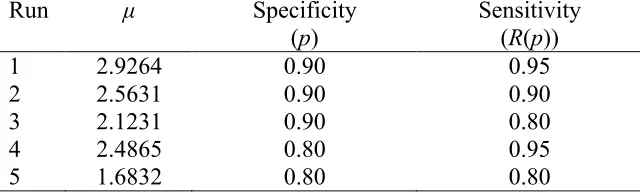
In the first simulation study, the distribution function F was chosen to be a

standard normal distribution whereas the distribution function G was a normal

distribution with mean μ and variance 1. The specificity was fixed at 80% or 90% level

for different values of μ (See Table I). The results of the simulation study at the nominal

level of 95% are given in Tables IV-IX.

Table I. Parameter settings for the normal distribution at fixed levels of specificity.

Run μ Specificity Sensitivity (p) (R(p))

1 2.9264 0.90 0.95

2 2.5631 0.90 0.90

3 2.1231 0.90 0.80

4 2.4865 0.80 0.95

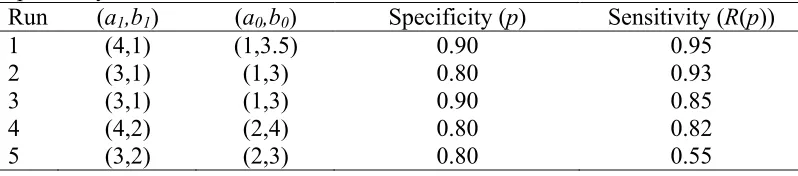
Our distributions, F and G, were beta distributions with parameters (a0,b0) and

(a1,b1) respectively in the second simulation study. The specificity was also fixed at 80%

or 90% for different values of (a0,b0) and (a1,b1) to get the corresponding sensitivities

(See Table II). The coverage probabilities resulting from the simulation study at the

nominal level of 95% are given in Tables X-XV.

Table II. Parameter setting for the Beta Distribution at fixed levels of specificity.

Run (a1,b1) (a0,b0) Specificity (p) Sensitivity (R(p))

1 (4,1) (1,3.5) 0.90 0.95

2 (3,1) (1,3) 0.80 0.93

3 (3,1) (1,3) 0.90 0.85

4 (4,2) (2,4) 0.80 0.82

5 (3,2) (2,3) 0.80 0.55

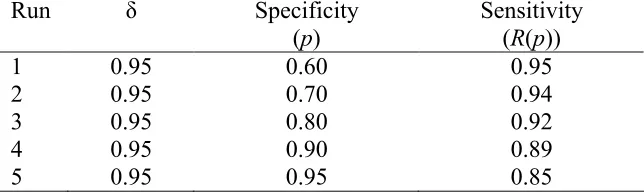
In the third simulation study, we chose the distributions F and G to be the

standard exponential distribution (with rate = 1) and an exponential distribution with rate

= 1/δ - 1, where δ represents the area under the receiver operating characteristic curve

(AUC). Here, δ was taken to be 0.95. Specificity was set at 0.60, 0.70, 0.80, 0.90 and

0.95 along with the corresponding sensitivities (See Table III). The coverage probabilities

resulting from the simulation study at the nominal level of 95% are given in Tables

Table III. Parameter settings for the exponential distribution

Run δ Specificity Sensitivity (p) (R(p))

1 0.95 0.60 0.95

2 0.95 0.70 0.94

3 0.95 0.80 0.92

4 0.95 0.90 0.89

5 0.95 0.95 0.85

The simulation studies illustrate that the newly proposed intervals generally

performed better than the normal approximation based interval at the 95% nominal level

Chapter VI

REAL APPLICATION

In this chapter, we apply the newly proposed intervals to a real life data example.

The data is from 403 subjects out of a group of 1046 who were selected to gain more

understanding regarding the prevalence of diabetes, obesity, etc. among African

Americans in central Virginia. The risk factors that were chosen from the study were the

waist and hip measurements, as they have been known to be a predictor of diabetes.

6.1 Detection of Diabetes

Diabetes is a disease resulting from the way our bodies use blood glucose. The

glucose (sugar) is your body’s energy source. Insulin, produced by the pancreas, helps the

body produce sugar, which is used for energy. Too little insulin or the body using it

improperly causes diabetes. It is the 5th leading cause of death in America and more

prevalent among African Americans. Left untreated, diabetes leads to amputations, organ

failure and even death in some cases.

Our study used the waist and hip measurements (in inches) of 388 female and

male subjects to determine the waist/hip ratio (WHR). The waist/hip ratio is just one way

of detecting diabetes in patients. Excess abdominal fat has been associated with higher

levels of insulin, which can raise blood sugar and pressure among other things. A WHR

patients. Snijder et al. (2004) found that waist and hip measurements are important

factors in predicting diabetes and other diseases.

The new empirical likelihood confidence intervals were applied to the data to

determine the accuracy of the WHR in predicting diabetes. There were 305 non-diseased

patients and 83 diseased patients. The results of the computation are found in Table XXII.

Chapter VII

DISCUSSION

Diagnostic testing is essential in distinguishing diseased patients from

non-diseased patients. When the result of a test is more accurate, there is less misconduct and

better treatment options can be implemented. The ROC curve provides a summary of the

performance of a diagnostic test (Claeskens et. al, 2003). For a quantitative test, the

cutoff point c is imperative because it determines which patients will be classified as

diseased and non-diseased. When the response of a test is continuous, it is of interest to

construct confidence intervals for the sensitivity of the test at this point. Calculating the

sensitivity and specificity of a test at various cutoff points is effective in determining the

best point at which to classify the test. The normal approximation confidence intervals

are inadequate when the distribution is skewed or the parameter range is restricted (Wu

and Rao, 2006). We proposed three new empirical likelihood confidence intervals for the

sensitivity of a continuous scale diagnostic test at a fixed level of specificity. The newly

proposed intervals were shown to generally perform better than the normal

REFERENCES

Claeskens G, Jing BY, Peng L, and Zhou W (2003). An empirical likelihood confidence interval for an ROC curve. The Canadian Journal of Statistics, 31: 173-190.

http://biostat.mc.vanderbilt.edu/twiki/bin/view/Main/DataSets

Linnet K (1987). Comparison of quantitative diagnostic tests: type I error, power, and sample size. Statistics in Medicine, 6: 147-158.

Metz CE (1978). Basic principles of ROC analysis, Sem Nuc Med., 8:283-298.

Owen A (1988). Empirical likelihood ratio confidence intervals for single functional.

Biometrika, 75: 237-249.

Owen A (1990). Empirical likelihood ratio confidence regions. Annals of Statistics, 18:

90-120.

Pepe MS (2003). The Statistical Evaluation of Medical Tests for Classification and Prediction. Oxford University Press, Cary, NC.

Platt RW, Hanley JA and Yang H (2000). Bootstrap confidence intervals for the sensitivity of a quantitative diagnostic test. Statistics in Medicine, 19: 313-322.

Qin GS (2006). Empirical likelihood based confidence intervals for the sensitivity of a continuous-scale diagnostic test at a fixed level of specificity. Manuscript. Department of Mathematics and Statistics. Georgia State University.

Qin GS, and Zhou XH (2006). Empirical likelihood inference for the area under the ROC curve. Biometrics,62: 613-622.

Shapiro DE (1999). The interpretation of diagnostic tests. Statistical Methods in Medical

Research, 8: 113-134

Snijder MB, Zimmet PZ, Visser M, Dekker JM, Seidell JC, and Shaw JE (2004). Independent and opposite associations of waist and hip circumferences with diabetes, hypertension and dyslipidemia: the AusDiab Study. International Journal of Obesity and

Related Metabolic Disorders, 28(3): 402-409.

Zhang Z and Pepe MS (2005), A Linear Regression Framework for Receiver Operating Characteristic(ROC) Curve Analysis. UW Biostatistics Working Paper Series. Working Paper 253.

Http://www.cdc.gov

Zhou XH, and Qin GS (2005). Improved confidence intervals for the sensitivity of a continuous-scale diagnostic test at a fixed level of specificity. Statistical in Medicine, 24:

465-477.

Altan AE, Carlson AM, Nettles A. The glycosolated hemoglobin as a diagnostic and monitoring tool for diabetes: evidence from claims data. AHSR FHSR Annu Meet Abstr

Book. 1996; 13: 11.

Zou KH, Hall WJ and Shapiro DE (1997). Smooth non-parametric receiver operating characteristic (ROC) curves for continuous diagnostic tests. Statistics in Medicine, 16:

APPENDIX I: SIMULATION TABLES

A. Normal Distribution Tables

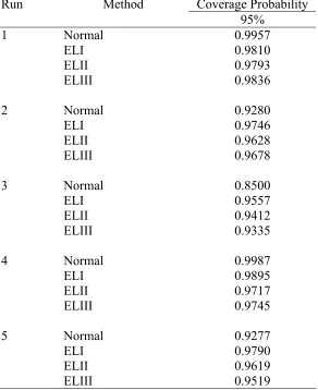
Table IV. Coverage probabilities of intervals at the nominal level of 95 percent when the data are generated from the normal distribution with m=20 and n=50.

Run Method Coverage Probability 95%

1 Normal 0.9957

ELI 0.9810

ELII 0.9793

ELIII 0.9836

2 Normal 0.9280

ELI 0.9746

ELII 0.9628

ELIII 0.9678

3 Normal 0.8500

ELI 0.9557

ELII 0.9412

ELIII 0.9335

4 Normal 0.9987

ELI 0.9895

ELII 0.9717

ELIII 0.9745

5 Normal 0.9277

ELI 0.9790

ELII 0.9619

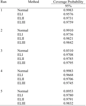
Table V. Coverage probabilities of intervals at the nominal level of 95 percent when the data are generated from the normal distribution with m=50 and n=20.

Run Method Coverage Probability 95%

1 Normal 0.9983

ELI 0.9576

ELII 0.9731

ELIII 0.9759

2 Normal 0.9910

ELI 0.9736

ELII 0.9821

ELIII 0.9842

3 Normal 0.8510

ELI 0.9708

ELII 0.9785

ELIII 0.9795

4 Normal 0.9983

ELI 0.9668

ELII 0.9706

ELIII 0.9745

5 Normal 0.8953

ELI 0.9780

ELII 0.9791

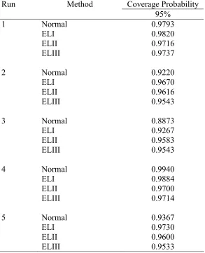
Table VI. Coverage probabilities of intervals at the nominal level of 95 percent when the data are generated from the normal distribution with m=50 and n=100. Run Method Coverage Probability

95%

1 Normal 0.9793

ELI 0.9820

ELII 0.9716

ELIII 0.9737

2 Normal 0.9220

ELI 0.9670

ELII 0.9616

ELIII 0.9543

3 Normal 0.8873

ELI 0.9267

ELII 0.9583

ELIII 0.9543

4 Normal 0.9940

ELI 0.9884

ELII 0.9700

ELIII 0.9714

5 Normal 0.9367

ELI 0.9730

ELII 0.9600

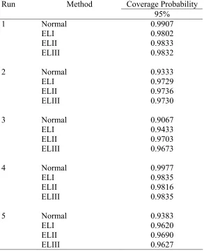
Table VII. Coverage probabilities of intervals at the nominal level of 95 percent when the data are generated from the normal distribution with m=100 and n=50. Run Method Coverage Probability

95%

1 Normal 0.9907

ELI 0.9802

ELII 0.9833

ELIII 0.9832

2 Normal 0.9333

ELI 0.9729

ELII 0.9736

ELIII 0.9730

3 Normal 0.9067

ELI 0.9433

ELII 0.9703

ELIII 0.9673

4 Normal 0.9977

ELI 0.9835

ELII 0.9816

ELIII 0.9835

5 Normal 0.9383

ELI 0.9620

ELII 0.9690

Table VIII. Coverage probabilities of intervals at the nominal level of 95 percent when the data are generated from the normal distribution with m=n=50.

Run Method Coverage Probability 95%

1 Normal 0.9947

ELI 0.9782

ELII 0.9798

ELIII 0.9844

2 Normal 0.9133

ELI 0.9771

ELII 0.9750

ELIII 0.9757

3 Normal 0.8853

ELI 0.9343

ELII 0.9637

ELIII 0.9567

4 Normal 0.9983

ELI 0.9859

ELII 0.9821

ELIII 0.9840

5 Normal 0.9313

ELI 0.9663

ELII 0.9646

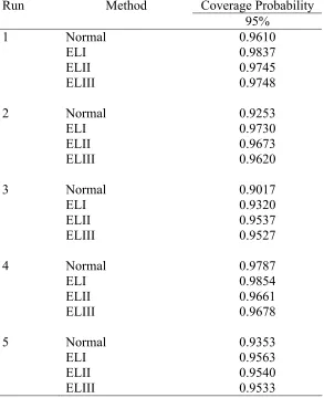
Table IX. Coverage probabilities of intervals at the nominal level of 95 percent when the data are generated from the normal distribution with m=n=100.

Run Method Coverage Probability 95%

1 Normal 0.9610

ELI 0.9837

ELII 0.9745

ELIII 0.9748

2 Normal 0.9253

ELI 0.9730

ELII 0.9673

ELIII 0.9620

3 Normal 0.9017

ELI 0.9320

ELII 0.9537

ELIII 0.9527

4 Normal 0.9787

ELI 0.9854

ELII 0.9661

ELIII 0.9678

5 Normal 0.9353

ELI 0.9563

ELII 0.9540

B. Beta Distribution Tables

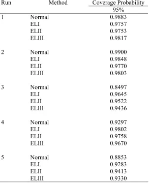
Table X. Coverage probabilities of intervals at the nominal level of 95 percent when the data are generated from the beta distribution with m=20 and n=50.

Run Method Coverage Probability 95%

1 Normal 0.9883

ELI 0.9757

ELII 0.9753

ELIII 0.9817

2 Normal 0.9900

ELI 0.9848

ELII 0.9770

ELIII 0.9803

3 Normal 0.8497

ELI 0.9645

ELII 0.9522

ELIII 0.9436

4 Normal 0.9297

ELI 0.9802

ELII 0.9758

ELIII 0.9670

5 Normal 0.8853

ELI 0.9283

ELII 0.9413

Table XI. Coverage probabilities of intervals at the nominal level of 95 percent when the data are generated from the beta distribution with m=50 and n=20.

Run Method Coverage Probability 95%

1 Normal 0.9957

ELI 0.9567

ELII 0.9671

ELIII 0.9726

2 Normal 0.9953

ELI 0.9702

ELII 0.9757

ELIII 0.9785

3 Normal 0.9457

ELI 0.9726

ELII 0.9823

ELIII 0.9827

4 Normal 0.9240

ELI 0.9724

ELII 0.9794

ELIII 0.9801

5 Normal 0.9023

ELI 0.9330

ELII 0.9603

Table XII. Coverage probabilities of intervals at the nominal level of 95 percent when the data are generated from the beta distribution with m=50 and n=100.

Run Method Coverage Probability 95%

1 Normal 0.9490

ELI 0.9760

ELII 0.9739

ELIII 0.9732

2 Normal 0.9697

ELI 0.9876

ELII 0.9705

ELIII 0.9685

3 Normal 0.8830

ELI 0.9363

ELII 0.9517

ELIII 0.9477

4 Normal 0.9380

ELI 0.9703

ELII 0.9527

ELIII 0.9470

5 Normal 0.9090

ELI 0.9220

ELII 0.9503

Table XIII. Coverage probabilities of intervals at the nominal level of 95 percent when the data are generated from the beta distribution with m=100 and n=50.

Run Method Coverage Probability 95%

1 Normal 0.9877

ELI 0.9752

ELII 0.9770

ELIII 0.9804

2 Normal 0.9657

ELI 0.9792

ELII 0.9751

ELIII 0.9764

3 Normal 0.8960

ELI 0.9503

ELII 0.9646

ELIII 0.9586

4 Normal 0.9360

ELI 0.9687

ELII 0.9650

ELIII 0.9573

5 Normal 0.9230

ELI 0.9330

ELII 0.9560

Table XIV. Coverage probabilities of intervals at the nominal level of 95 percent when the data are generated from the beta distribution with m=n=50.

Run Method Coverage Probability 95%

1 Normal 0.9817

ELI 0.9702

ELII 0.9744

ELIII 0.9767

2 Normal 0.9800

ELI 0.9841

ELII 0.9789

ELIII 0.9813

3 Normal 0.8847

ELI 0.9558

ELII 0.9648

ELIII 0.9615

4 Normal 0.9260

ELI 0.9696

ELII 0.9616

ELIII 0.9566

5 Normal 0.9070

ELI 0.9290

ELII 0.9547

Table XV. Coverage probabilities of intervals at the nominal level of 95 percent when the data are generated from the beta distribution with m=n=100.

Run Method Coverage Probability 95%

1 Normal 0.9370

ELI 0.9762

ELII 0.9708

ELIII 0.9684

2 Normal 0.9573

ELI 0.9853

ELII 0.9675

ELIII 0.9651

3 Normal 0.8960

ELI 0.9370

ELII 0.9587

ELIII 0.9530

4 Normal 0.9520

ELI 0.9667

ELII 0.9623

ELIII 0.9590

5 Normal 0.9227

ELI 0.9320

ELII 0.9507

C. Exponential Distribution Tables

Table XVI. Coverage probabilities of intervals at the nominal level of 95 percent when the data are generated from the exponential distribution with m=20 and n=50. Run Method Coverage Probability

95%

1 Normal 0.9993

ELI 0.9837

ELII 0.9783

ELIII 0.9791

2 Normal 0.9940

ELI 0.9875

ELII 0.9811

ELIII 0.9840

3 Normal 0.9423

ELI 0.9860

ELII 0.9818

ELIII 0.9846

4 Normal 0.8893

ELI 0.9815

ELII 0.9737

ELIII 0.9690

5 Normal 0.8357

ELI 0.9369

ELII 0.9452

Table XVII. Coverage probabilities of intervals at the nominal level of 95 percent when the data are generated from the exponential distribution with m=50 and n=20. Run Method Coverage Probability

95%

1 Normal 0.9983

ELI 0.9771

ELII 0.9766

ELIII 0.9776

2 Normal 0.9977

ELI 0.9493

ELII 0.9620

ELIII 0.9638

3 Normal 0.9950

ELI 0.9723

ELII 0.9733

ELIII 0.9729

4 Normal 0.9677

ELI 0.9770

ELII 0.9788

ELIII 0.9800

5 Normal 0.9733

ELI 0.9694

ELII 0.9729

Table XVIII. Coverage probabilities of intervals at the nominal level of 95 percent when the data are generated from the exponential distribution with m=50 and n=100. Run Method Coverage Probability

95%

1 Normal 0.9616

ELI 0.9899

ELII 0.9689

ELIII 0.9448

2 Normal 0.9520

ELI 0.9873

ELII 0.9669

ELIII 0.9599

3 Normal 0.9467

ELI 0.9850

ELII 0.9643

ELIII 0.9567

4 Normal 0.9363

ELI 0.9653

ELII 0.9647

ELIII 0.9597

5 Normal 0.9130

ELI 0.9337

ELII 0.9457

Table XIX. Coverage probabilities of intervals at the nominal level of 95 percent when the data are generated from the exponential distribution with m=100 and n=50. Run Method Coverage Probability

95%

1 Normal 0.9773

ELI 0.9709

ELII 0.9764

ELIII 0.9768

2 Normal 0.9806

ELI 0.9867

ELII 0.9765

ELIII 0.9779

3 Normal 0.9063

ELI 0.9763

ELII 0.9736

ELIII 0.9763

4 Normal 0.9087

ELI 0.9625

ELII 0.9678

ELIII 0.9655

5 Normal 0.9127

ELI 0.9489

ELII 0.9619

Table XX. Coverage probabilities of intervals at the nominal level of 95 percent when the data are generated from the exponential distribution with m=n=50.

Run Method Coverage Probability 95%

1 Normal 0.9907

ELI 0.9870

ELII 0.9759

ELIII 0.9773

2 Normal 0.9850

ELI 0.9838

ELII 0.9764

ELIII 0.9792

3 Normal 0.9147

ELI 0.9793

ELII 0.9793

ELIII 0.9806

4 Normal 0.9097

ELI 0.9695

ELII 0.9709

ELIII 0.9702

5 Normal 0.9020

ELI 0.9375

ELII 0.9469

Table XXI. Coverage probabilities of intervals at the nominal level of 95 percent when the data are generated from the exponential distribution with m=n=100.

Run Method Coverage Probability 95%

1 Normal 0.9397

ELI 0.9807

ELII 0.9582

ELIII 0.9548

2 Normal 0.9323

ELI 0.9799

ELII 0.9655

ELIII 0.9592

3 Normal 0.9523

ELI 0.9687

ELII 0.9563

ELIII 0.9543

4 Normal 0.9207

ELI 0.9550

ELII 0.9577

ELIII 0.9540

5 Normal 0.9247

ELI 0.9463

ELII 0.9580

APPENDIX II: REAL APPLICATION TABLE

Table XXII. Confidence Intervals for R(p) for the real data application at the 95% nominal level.

Specificity Method Sensitivity Confidence Intervals Length

(p) R(p)

0.95 ELI 0.1446 (0.0714, 0.2473) .1759 ELII 0.1446 (0.0591, 0.2741) .2150 ELIII 0.1446 (0.0590, 0.2742) .2152

0.90 ELI 0.2410 (0.1457, 0.3576) .2119 ELII 0.2410 (0.1521, 0.3480) .1959 ELIII 0.2410 (0.1505, 0.3503) .1998

0.85 ELI 0.3133 (0.2055, 0.4366) .2311 ELII 0.3133 (0.1989, 0.4454) .2465 ELIII 0.3133 (0.1983, 0.4462) .2479

0.80 ELI 0.4096 (0.2920, 0.5347) .2427 ELII 0.4096 (0.2864, 0.5410) .2546 ELIII 0.4096 (0.2857, 0.5419) .2562

APPENDIX III: S-PLUS CODE FOR SIMULATION

# Computing the pseudo empirical likelihood ratio confidence intervals for ROC curve

#

# December 3, 2005 #

###############################################################################

m<-20 n<-50

#sp<-0.7 # 0.90, 0.80, 0.70 iter<-3000

levelc1<-0.90 levelc2<-0.95

############################################################################ #normal distribution.

#muy<-1 # the mean of diseased population #sens<-1-pnorm(qnorm(sp),muy,1)

#sp = 0.9; muy = 2.9264 #sp = 0.9; muy = 2.5631 #sp = 0.9; muy = 2.1231 #sp = 0.8; muy = 2.4865 #sp = 0.8; muy = 1.6832

#sens<-1-pnorm(qnorm(sp),muy,1)

############################################################################ #Exponential distribution.

#sp<- 0.95 # specificity = 0.6, 0.7, 0.8, 0.9, 0.95 #delta<- 0.95 # AUC = 0.95

#sens<- 1-pexp(qexp(sp), rate= (1/delta -1)) ############################################################################

########################################################################### #Beta(a,b) distribution.

#Table 2:

#Run 1: specificity=1-tt=0.9, sensitivity=0.95

#sp<-0.9; a0<-1; b0<-3.5; a1<-4; b1<-1;# sensitivity=0.946002

# Delete the "#" before "tt" when you run "Run 1" for Beta(a,b) distribution.

#Run 2: specificity=1-tt=0.8, sensitivity=0.93

#sp<-0.8; a0<-1; b0<-3; a1<-3; b1<-1; # sensitivity=0.9284251

# Delete the "#" before "tt" when you run "Run 2" for Beta(a,b) distribution.

#sp<-0.9; a0<-1; b0<-3; a1<-3; b1<-1; # sensitivity=0.8461462

# Delete the "#" before "tt" when you run "Run 3" for Beta(a,b) distribution.

#Run 4: specificity=1-tt=0.8, sensitivity=0.82

#sp<-0.8; a0<-2; b0<-4; a1<-4; b1<-2; # sensitivity=0.8245191

# Delete the "#" before "tt" when you run "Run 4" for Beta(a,b) distribution.

#Run 5: specificity=1-tt=0.8, sensitivity=0.55

#sp<-0.8; a0<-2; b0<-3; a1<-3; b1<-2; # sensitivity=0.5548815

# Delete the "#" before "tt" when you run "Run 5" for Beta(a,b) distribution.

#sens<- 1-pbeta(qbeta(sp,a0,b0),a1,b1) #sensitivity

# Delete the "#" before "Rtt" when you run the S code for Beta(a,b) distribution.

############################################################################

p<-1-sp

coverage1<-0 coverage2<-0

coverageb11<-0 # First bootstrap coverageb12<-0

coverageb21<-0 # Second bootstrap coverageb22<-0

coveraget1<-0 coveraget2<-0

CILT1<-c(rep(0,iter)) CILT2<-c(rep(0,iter))

# Loop

Rp<-0

for ( i in c(1:iter)) {

#normal distribution:

#x<-rnorm(m,0,1) # obs from non-diseased population #y<-rnorm(n,muy,1) # obs from diseased population

#Exponential distribution: rexp(n, rate=1, scale)

#x<-rexp(m, rate= 1) # obs from non-diseased population #y<-rexp(n, rate= (1/delta -1)) # obs from diseased population

#Beta(a,b) distribution:

#x<-rbeta(m,a0,b0) #nondesease:

# Delete the "#" before "x" when you run the S code for Beta(a,b) distribution.

# Delete the "#" before "y" when you run the S code for Beta(a,b) distribution.

u<-rep(100,n) # hat U =1- hat F for (j in 1:n)

{

u[j]<-1-mean((x<=y[j])) }

indU<-(u <= p)*1 # indicator function of U: I(U_j <=p)

Rp[i]<-mean(indU)

# compute the scale constant c(p). if ((Rp[i]!=1) & (Rp[i]!=0))

{

sigma<-Rp[i]*(1-Rp[i]) # estimate for sigma^2

hg<-bandwidth.sj(y, nb=1000, method="dpi") # Uses the method of Sheather & Jones (1991)

# to select the bandwidth of a Gaussian kernel density estimator for g

hf<-bandwidth.sj(x, nb=1000, method="dpi") # Uses the method of Sheather & Jones (1991)

# to select the bandwidth of a Gaussian kernel density estimator for f

quantileF<-quantile(x,1-p)

densityg<-density(y,n=1,window="g",width=hg, from=quantileF)$y #density(.): density estimate at (1-p)-th quantile of F.

densityf<-density(x,n=1,window="g",width=hf, from=quantileF)$y #density(.): density estimate at tt-th quantile of F.

hatsigma1<-sigma + n*p*(1-p)*densityg/(m*densityf) # estimate for sigma_1^2

#sigma1<-sigma + n*p*(1-p)*dnorm(qnorm(1-p), muy, 1)/(m*dnorm(qnorm(1-p),0,1))

# True value of sigma_1^2

#bootstrap estimates for R(p). Bootstap variance estimate of R(p) test<-sensb(y,x,1-p,300,0) Rpboot<-mean(test) Rpvar<-var(test) cp<-sigma/hatsigma1 cpstar1<- sigma/(n*Rpvar) cpstar2<- Rpboot*(1-Rpboot)/(n*Rpvar)

# cat("the scale constant cp=",cp, "\n") wjhat<-indU-sens

funclambda<-function(lam)mean(wjhat/(1+lam*wjhat)) lambda<-solveNonlinear(funclambda, c(0), c(0.01))$x #lambda<-sum(wjhat)/sum(wjhat^2)

coverage1[i]<-(cp*lroc <= qchisq(levelc1,1))*1 coverage2[i]<-(cp*lroc <= qchisq(levelc2,1))*1

coverageb11[i]<-(cpstar1*lroc <= qchisq(levelc1,1))*1 # First bootstrap

coverageb12[i]<-(cpstar1*lroc <= qchisq(levelc2,1))*1

coverageb21[i]<-(cpstar2*lroc <= qchisq(levelc1,1))*1 # second bootstrap

coverageb22[i]<-(cpstar2*lroc <= qchisq(levelc2,1))*1

}else{

coverage1[i]<-NA; coverage2[i]<-NA coverageb11[i]<-NA; coverageb12[i]<-NA coverageb21[i]<-NA; coverageb22[i]<-NA }

# compute the normal approximation based interval.

hwidth1<-qnorm(1-(1-levelc1)/2)*(hatsigma1/n)^(1/2) tlow1<-Rp[i]-hwidth1 # lower limit of the CI tup1<- Rp[i]+hwidth1 # upper limit of the CI

if ((tlow1 <= sens) & (tup1 >= sens))coveraget1<-coveraget1+1 CILT1[i]<-2*hwidth1 # The length of CI

hwidth2<-qnorm(1-(1-levelc2)/2)*(hatsigma1/n)^(1/2) tlow2<-Rp[i]-hwidth2 # lower limit of the CI tup2<- Rp[i]+hwidth2 # upper limit of the CI

if ((tlow2 <= sens) & (tup2 >= sens))coveraget2<-coveraget2+1 CILT2[i]<-2*hwidth2 # The length of CI

}

sink("pseudoelroc1bootres")

#Normal distribution: # Delete the "#"'s before "cat" when you run the S code for normal distribution.

#cat("Normal distribution: m=", m, "n=", n, "specificity=", sp, "sensitivity=", sens, "mu=", muy, "iter=", iter, "\n")

#Exponential distribution: # Delete the "#"'s before "cat" when you run the S code for Exponential distribution.

#cat("Exponential dist: m=", m, "n=", n, "sp=", sp, "sens=", sens, "AUC=", delta, "iter=", iter, "\n")

# Beta distribution: # Delete the "#"'s before "cat" when you run the S code for Beta distribution.

#cat("Beta distribution: m=", m, "n=", n, "iter=", iter, "\n")

#cat("specifity=",sp, "sens=", sens, "a0=",a0,"a1=",a1,"b0=",b0,"b1=",b1, "\n")

cat("CI for sensitivity at level=", levelc1, "\n")

cat("Coverage of the ELRCI :", mean(sort(coverage1)), "\n")

cat("second bootstrap method. Coverage of the ELRCI :", mean(sort(coverageb21)), "\n")

cat("Coverage of the Normal CI :", coveraget1/iter, "\n")

#cat("Average length of ELRCI: ", mean(CIL), " STD=", (var(CIL))^(1/2), "\n") cat("Average length of Normal CI: ", mean(CILT1), " STD=",

(var(CILT1))^(1/2), "\n")

#cat("Midpoint:", mean(Mid), " STD=", (var(Mid))^(1/2), "\n")

cat("---","\n")

cat("CI for sensitivity at level=", levelc2, "\n")

cat("Coverage of the ELRCI :", mean(sort(coverage2)), "\n")

cat("First bootstrap method. Coverage of the ELRCI :", mean(sort(coverageb12)), "\n")

cat("second bootstrap method. Coverage of the ELRCI :", mean(sort(coverageb22)), "\n")

cat("Coverage of the Normal CI :", coveraget2/iter, "\n")

#cat("Average length of ELRCI: ", mean(CIL), " STD=", (var(CIL))^(1/2), "\n") cat("Average length of Normal CI: ", mean(CILT2), " STD=",

(var(CILT2))^(1/2), "\n")

#cat("Midpoint:", mean(Mid), " STD=", (var(Mid))^(1/2), "\n")

cat("Mean estimate for sensitivity:", mean(Rp), " STD=", (var(Rp))^(1/2), "\n")

APPENDIX IV: S-PLUS CODE FOR REAL APPLICATION

# Computing the pseudo empirical likelihood ratio confidence intervals for ROC curve

#

# Jan. 3, 2006

#Diabetes example

xx<-NON[,1] # obs from non-diseased population yy<-DIS[,1] # obs from diseased population

x<-sort(xx) y<-sort(yy)

m<-length(x) n<-length(y)

levelc<-0.95

crit<-qchisq(levelc,1)

sp<- 0.95 # specificity

p<-1-sp # p<-1-sp # False Positive Rate

ELlow<-0 # EL interval ELup<-0

BELlow1<-0 # First bootstrap EL-based CI BELup1<-0

BELlow2<-0 # Second bootstrap EL-based CI BELup2<-0

u<-rep(100,n) # hat U =1- hat F for (j in 1:n)

{

u[j]<-1-mean((x<=y[j])) }

hg<-bandwidth.sj(y, nb=1000, method="dpi") # Uses the method of Sheather & Jones (1991)

# to select the bandwidth of a Gaussian kernel density estimator for g hf<-bandwidth.sj(x, nb=1000, method="dpi")

# Uses the method of Sheather & Jones (1991)

# to select the bandwidth of a Gaussian kernel density estimator for f

indU<-(u <= p)*1 # indicator function of U: I(U_j <=p)

Rp<-mean(indU) # estimate for R(p). Sensitivity

# compute the scale constant c(p).

sigma<-Rp*(1-Rp) # estimate for sigma^2

densityg<-density(y,n=1,window="g",width=hg, from=quantileF)$y #density(.): density estimate at (1-p)-th quantile of F. densityf<-density(x,n=1,window="g",width=hf, from=quantileF)$y #density(.): density estimate at tt-th quantile of F.

hatsigma1<-sigma + n*p*(1-p)*densityg^2/(m*densityf^2) # estimate for sigma_1^2

#bootstrap estimates for R(p). Bootstap variance estimate of R(p)

test<-sensb(y,x,1-p,1000,0) Rpboot<-mean(test)

Rpvar<-var(test)

cp<-sigma/hatsigma1 cpstar1<- sigma/(n*Rpvar)

cpstar2<- Rpboot*(1-Rpboot)/(n*Rpvar)

# cat("the scale constant cp=",cp, "\n")

critcp_crit/cp # EL interval

critcps1_crit/cpstar1 # First bootstrap EL-based CI

critcps2_crit/cpstar2 # second bootstrap EL-based CI

# EL confidence intervals

y<-elciroc(n,indU,critcp) # calling "elciroc" to compute the EL interval.

ELlow<-y[4] # lower limit of the EL CI

ELup<-y[5] # upper limit of the EL CI

# first bootstrap EL based CI:

y<-elciroc(n,indU,critcps1) # calling "elciroc" to compute the EL interval.

BELlow1<-y[4] # lower limit of the bootstrap EL CI BELup1<- y[5] # upper limit of the bootstrap EL CI

# Second bootstrap EL based CI:

y<-elciroc(n,indU,critcps2) # calling "elciroc" to compute the EL interval.

BELlow2<-y[4] # lower limit of the bootstrap EL CI BELup2<- y[5] # upper limit of the bootstrap EL CI

sink("realexampleres")

cat("CI for sens at level=", levelc, "m=", m, "n=", n, "\n") cat("specificity =", sp, "\n")

cat("R(p)=", Rp, "\n")

cat("upper limit of the EL CI :", ELup, "\n")

cat("lower limit of the First bootstrap EL CI :", BELlow1, "\n") cat("upper limit of the First bootstrap EL CI :", BELup1, "\n")

cat("lower limit of the second bootstrap EL CI :", BELlow2, "\n") cat("upper limit of the second bootstrap EL CI :", BELup2, "\n")

cat("---","\n")