PRL RR 1 pdf

Incremental Computation of Planar Maps

Michel Gangnet

Jean-Claude Herv ´e Thierry Pudet

Jean-Manuel Van Thong

This report is a revised and extended version of the paper entitled ‘Incremental Computation of Planar Maps’, by the same authors, published in the SIGGRAPH’89 Conference Proceedings.

c

Digital Equipment Corporation 1991

A planar map is a figure formed by a set of intersecting lines and curves. Such an object captures both the geometrical and the topological information implicitly defined by the data. In the context of 2D drawing, it provides a new interaction paradigm, map sketching, for editing graphic shapes. To build a planar map, one must compute curve intersections and deduce from them the map they define. The computed topology must be consistent with the underlying geometry. Robustness of geometric computations is a key issue in this process. This report presents a robust solution to B´ezier curve intersection that uses exact forward differencing and bounded rational arithmetic. Data structures and algorithms supporting incremental insertion of B´ezier curves in a planar map are described. A prototype illustration tool using this method is also discussed.

R ´esum ´e

B´ezier curves, forward differences, curve intersection, rational arithmetic, planar maps, map sketching.

Acknowledgements

2 Map Sketching 2

3 B ´ezier Curve Interpolation and Intersection 4

3.1 Overview

: : : : : : : : : : : : : : : : : : : : : : : : : : : : : : : : : :

5 3.2 Interpolation Method

: : : : : : : : : : : : : : : : : : : : : : : : : : : :

6 3.3 Intersection Algorithm

: : : : : : : : : : : : : : : : : : : : : : : : : : :

8 3.4 Topology Consistency

: : : : : : : : : : : : : : : : : : : : : : : : : : :

9

4 Data Structure and Algorithms 11

4.1 Planar Map Description

: : : : : : : : : : : : : : : : : : : : : : : : : :

11 4.2 Polycurve Insertion

: : : : : : : : : : : : : : : : : : : : : : : : : : : :

13 4.3 Updating the Inclusion Tree

: : : : : : : : : : : : : : : : : : : : : : : :

14 4.4 Point Location

: : : : : : : : : : : : : : : : : : : : : : : : : : : : : : :

15

5 Conclusion 16

1 Introduction

There is growing interest in the robustness of geometric computations [9, 5, 13]. Different graphics algorithms have different sensitivity to numerical errors. In some cases, numerical errors are acceptable. In others, one can find ways around them. However, exact computation is sometimes mandatory. The following examples demonstrate the range of effects.

[image:7.612.122.445.381.531.2]

When scan–converting 3D polygons, rounding errors on face equations will not prevent the z–buffer method from rendering a scene. The few erroneous pixels may not even be visible. This is a case where numerical errors are innocuous. A second example is a function performing point location in a polygon with a parity test, using floating point arithmetic. If the result returned by this function is used for identification of the polygon and, say, modification of its color, then it is acceptable for the function to return an empty result when a reliable answer cannot be computed. Hence, in some 2D drawing programs, the user must click well inside a polygon to select it (which is better than selecting the wrong polygon). As a third example consider a program implementing an algorithm which presumes infinite precision. The Bentley–Ottmann algorithm [3, 20] for reporting intersections of a set of non–vertical line segments relies on the fact that two segments may intersect iff there exists a position of the vertical sweep–line where they are consecutive. If the implementation produces an error when inserting a new segment in the sweep–line then some intersections may be missed. In this case, it is imperative to provide an exact answer.

Figure 1: A planar map.

studied by numerous researchers [20, 12, 7]. It is standard practice to distinguish between the geometry, that is the position of the vertices and the geometric definition of the edges, and the topology, that is the incidence and adjacency of the vertices, edges, and faces.

The problem addressed here is building a data structure to support incremental insertion of new curves in a planar map, dynamically computing new intersections and updating the data structure. In this case, topological information has to be deduced from geometrical information. When two curves intersect at a new vertex, the ordering of the four edges around the vertex provides topological information used to follow the contour of a face incident to the vertex. If floating point arithmetic is used, it has been shown that the computed slopes can give the wrong order [9, 18]. This is similar to the Bentley–Ottmann algorithm example above.

Our first implementation [19] used the Bentley–Ottmann algorithm and rational arithmetic to compute the planar map formed by a set of line segments; [10] is the description of a 2D illustration tool based on this first software. The method was not incremental and the map had to be recomputed each time a new segment was added. In [11], Greene and Yao solve the intersection problem for line segments by working directly in the discrete plane. In [8], Edelsbrunner et al. study arrangements of Jordan curves in the plane from a theoretical point of view.

In the next section, the utility of planar maps for 2D drawing is briefly discussed. Section 3 details curve intersection. First, B´ezier curves are interpolated by polylines using forward differencing. Then, the intersection between two interpolating polylines is computed with rational arithmetic; we show how it is possible to limit the number of bits in this process and how to control the quality of the interpolation. Section 4 describes the map data structure and the two main algorithms used in the planar map construction process: incremental insertion of a curve and point location in a map. The map topology is computed from the geometry of the polylines. Since exact arithmetic is used in this process, the map topology, although it may be different from the topology defined by the true curves, is always consistent with the geometry of the interpolating polylines.

2 Map Sketching

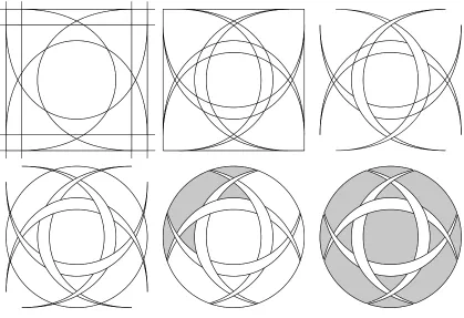
Our interest in planar maps is motivated by practical concerns: with traditional graphic arts media (pencil, eraser, ink, etc.), it is common practice to build shapes by drawing lines and curves, erase some pieces thereof, and color or ink the areas they delimit (see [1] and Fig. 2). The design of logos and monograms, floor plan sketching by architects, and cartoon cell drawing and inking are examples where this technique is used. In typical drawing software there is no way to mimic this method. If Fig. 3a is drawn by the user of a drawing application as four lines, it is impossible for him to color the rectangle (as in Fig. 3b) since no such rectangle exists. If the drawing were computed as a planar map, this dual interpretation would be possible.

[image:9.612.86.475.132.285.2]

Figure 2: Graphic design by space division (B. Munari in [1]).

a b

of three basic steps: drawing, erasing, and coloring. We call this technique map sketching and have implemented it in prototype illustration software used to draw the figures in this report. Fig. 4 illustrates map sketching. Strokes drawn by the user are incrementally added to the map describing the drawing. Two additional operations are allowed on a map: edge erasing and face coloring, using point location in a map. These steps can be iterated in any order.

[image:10.612.88.507.244.531.2]

Map sketching closely parallels the traditional pencil and eraser method and is more natural and more efficient for constructing certain classes of drawings. An illustration is described as an ordered set of maps, painted in back to front order. As a map can have transparent faces, shapes with holes may be defined. User interface design issues in map–based illustration software are further discussed in [2].

Figure 4: Map sketching.

3 B ´ezier Curve Interpolation and Intersection

polycurves; a polycurve is a list of B´ezier curves of degree greater than or equal to one such that the last control point of a curve is equal to the first control point of the next one. Polycurves can be either open or closed. A polycurve has a natural parameterization defined by the parameterization of its components. Inserting polycurves instead of curves also avoids creating unnecessary vertices of degree 2 in the description of the map topology. If a graphics primitive is made of several polycurves (e.g. the outline of the character O), these are grouped as one object at the application level.

3.1 Overview

The incremental insertion algorithm (Sec. 4) has two requirements. First, intersection points must be ordered without error along a polycurve by their parameter values, including the case of self-intersection. Second, if two or more polycurves intersect at one point, they must be ordered without error around the intersection. This ordering is used to follow the boundaries of the faces. To meet these requirements, we use the following strategy:

The control points of the B´ezier polycurves have integer coordinates on a grid large enough for 2D graphics applications. Grid size is discussed in Sec. 3.4.

The polycurve is replaced with an interpolating polyline. The polyline parameterization is defined by a one-to-one mapping of the polycurve on the polyline. We compute an exact interpolation of the polycurve by exact forward differencing. There must be enough bits available to perform forward differencing without a loss of precision (Sec. 3.2). Rather than storing polylines in the data structure, they are computed as needed. Some of the polylines may be cached.

Computing the intersection of two exact polylines causes an explosion in the number of bits (Sec. 3.4). Thus, we round the points of an exact polyline to the grid. Then the intersection of two rounded polylines is essentially the intersection of line segments whose endpoints have integer coordinates. Ordering two intersection points along the same line segment or ordering two intersecting line segments around their intersection point is done with rational arithmetic. Note that the intersection points are not rounded since this could modify the map topology.

Finally, it is natural with the map sketching technique to use an existing intersection point as a new polycurve endpoint. We show how to achieve this without increasing the bit length of the arithmetic (Sec. 3.4).

3.2 Interpolation Method

A polynomial B´ezier curve of degree

d

is defined by:

V

(

t

) =

d

X

r

=0

V

r

B

dr

(

t

)

;

0

t

1

;

where the

V

r

are the

d

+ 1 control points that form the control polygon of

V

(

t

), and

B

dr

(

t

) =

d

_r

!

t

r

₍₁

_t

₎

d r

is the

r

th Bernstein polynomial of degree

d

[21, 4].

Let k

v

k = max (j

x

v

j

;

j

y

v

j), where

v

is a vector in the Euclidean plane. For

d

2, the diagonal

D

and the length

L

of the control polygon of

V

(

t

) are defined as:

D

= max

0

r

d

2

k

V

r

+2 2

V

r

+1+

V

r

k

;

L

= max

0

r

d

1

k

V

r

+1

V

r

k

:

Wang [26, 23] gives the following result. If the de Casteljau subdivision algorithm (midpoint case) is applied down to depth

k

to a polynomial B´ezier curve of degree

d

2 with control points

V

r

, with:

k

=

log₄

d

(

d

1) 8

D

;

(1)

then all the chords (straight line segments) joining the endpoints of the 2

k

control polygons which are the leaves of the subdivision tree are closer to the curve than the threshold

. Since reference [26] is not available to us, an independent proof of this result is given below, together with a bound on the chord length.

Computing the first and second derivatives of

V

(

t

) and using the properties of the Bernstein polynomials gives, for all

t

in [0

;

1]:

k

V

(2)₍

t

₎

k

d

(

d

1)

D;

(2)

k

V

(1)₍

t

₎

k

d L:

(3)

To find the number of subdivisions, we use a chord interpolation theorem [22] which states that if

f

(

t

) is a real–valued function of class

C

∞on [

a;b

], then for all

t

in [

a;b

] :

j

f

(

t

)

s

(

t

)j

(

b a

)2 8

a

max

t

b

f

(2)₍

t

₎

;

(4)

Let

, 0

<

1, be a step size on the interval [0

;

1] and

n

the integer such that

n

= 1. This defines

n

intervals

I

i

= [

i;

(

i

+ 1)

], and

n

chords

S

i

(

t

) with endpoints

E

i

=

V

(

i

) and

E

i

+1 =

V

((

i

+ 1)

). Let

be a given threshold measuring the maximum allowed deviation

between the curve and the chords

S

i

. We want to ensure that:

k

V

(

t

)

S

i

(

t

)k

(5)

holds for all

i

, 0

i < n

, and all

t

in

I

i

.

Applying (4) to the coordinates of

V

(

t

) on the interval

I

i

and using the bound (2), it is straightforward to see that any

1 such that:

0

<

2 8

d

(

d

1)

D

(6)

will satisfy (5).

Let

k

be the smallest integer such that

= 2

k

satisfies (6), then:

k

=

log₄

d

(

d

1) 8

D

:

Equation (1) is cited in [23] as a result derived by Wang.

We can now bound the length of the chords given by a priori subdivision of depth

k

. The mean value theorem applied to

V

(

t

) on interval

I

i

gives:

k

E

i

+1

E

i

k

max

t

∈

I

i k

V

(1)₍

t

₎

k

:

The maximum ofk

V

(1)₍

t

₎

k over

I

i

is less than or equal to its maximum over [0

;

1]. Using (3), one getsk

E

i

+1

E

i

k

dL

. The bound on

from (6) gives for all

i

, 0

i <

2

k

:

k

E

i

+1

E

i

k s 8

d

d

1

L

p

D

p

:

(7)

Consider the chord endpoints

E

i

;

0

i

2

k

. They form a polyline

E

. It is faster to use ordinary forward differencing [16] than de Casteljau subdivision to compute

E

. Since a priori subdivision computes the complete tree to depth

k

, forward differencing with fixed step size 2

k

will generate the same polyline, provided that exact computations are done in both cases.

We now show that the number of bits needed to perform exact forward differencing is bounded. Suppose that the control points of a B´ezier curve have coordinates coded into

b

bits. Then, computing the subdivision tree down to depth

k

requires at most

b

+

kd

bits for the coordinates of the

E

i

. In the forward differencing loop, the only values involved in the

i

th iteration are the forward differences∆

j

E

i

, 0

j

d

. Since we know from subdivision that, for all

i

, the computation of

E

i

=∆0

E

i

requires at most

b

+

kd

bits,∆

j

E

i

requires at most

To limit the total number of bits needed when updating a planar map, the intersection algorithm uses rounded polylines. The exact coordinates of the

E

i

are computed by forward differencing each curve in a polycurve. They are then rounded to

b

bits. The rounded polyline associated with a given polycurve is the concatenation of the polylines associated with the curves in the polycurve. If there are line segments in the polycurve, they are added to the polyline without further processing.

Thus, given a polycurve

C

= (

C

i

;

0

i

n

), where the

C

i

are B´ezier curves defined by control points with integer coordinates, the method described above associates with it a rounded polyline

P

= (

P

i

;

0

i

m

) such that each chord on the polyline is closer to the corresponding section of

C

than the threshold

. As it is necessary to associate a parameterization of

P

with the natural one on

C

, each point

P

i

is defined by its coordinates, the curve index on

C

, and the value of the parameter

t

on the corresponding curve. As these last values are always dyadic numbers, it is enough to note the chord index. The chord index must be recorded because rounding may create chords with a null length, which are not stored in the polyline.

3.3 Intersection Algorithm

B´ezier curve intersection is studied by Sederberg and Parry [23]. In two of the algorithms they consider, rejection of non-intersecting pieces of two curves is done by bounding box comparison. Forward differencing is not convenient for successive midpoint evaluations of a curve. To take advantage of bounding boxes, a preprocessing step breaks the rounded polylines into monotonic pieces. For such a piece, the box of any subpiece is given by its endpoints coordinates. This method is also used by Koparkar and Mudur [14] with another curve evaluation method. In planar map construction, a new polycurve is intersected with a subset of the polycurves already inserted in the map. The preprocessing of the new polycurve finds the monotonic pieces, saving data to be used in later computations. The new polycurve is then immediately inserted in the map.

Preprocessing. Let

C

be the new polycurve, a) use the interpolation method to compute the points of the exact polyline

E

and of the rounded polyline

P

of

C

, b) store the points of

P

in an array, to be discarded after the insertion of

C

, c) find the monotonic pieces of

P

, d) at the end of a monotonic piece, save the permanent data associated with it, that is, its first and last indices (

i

f

;i

l

) on the polyline, its bounding box, its octant, and the forward differencing context at

i

f

(i.e., ∆

j

E

i

f

, for all

j

). The bounding box of

P

is also computed. These steps can be performed during the forward differencing loop. Different polycurves can be processed in parallel.

G

, and store the result into an array. Then, search the intersecting chords using binary subdivision on the respective arrays (the box of any subset of points considered in this subdivision is given by its two endpoints and the octant information). It is also possible to use linear search on both arrays.

In the map sketching application, the existing curve

G

may be partially erased. In this case only the monotonic pieces containing a non-erased part of

G

are intersected with

C

. Different pairs of intersecting pieces can be processed in parallel.

Since two polylines may be partially or totally overlapping (e.g. the case of two abutting rectangles), all intersections between two monotonic pieces are not transverse. To handle this case, the intersection algorithm returns an intersection context which describes the common interval on the two polylines (a closed interval in the transverse case), the parameters of its endpoints on the two polylines, and the ordering of the two polylines around each endpoint of the interval.

After preprocessing, a new curve is intersected with itself to detect multiple points and self-overlapping. It is worthwhile to cache partially– or totally–generated polylines. Two cases are frequent: a) the same monotonic piece of

G

intersects different pieces of

C

, and b) successive new polycurves intersect the same existing one.

3.4 Topology Consistency

This section describes how a consistent topology is obtained from the geometric data given by the intersection process. For illustration software, the input can be rounded to an integer grid if the grid size is large enough. A typical case is to output the results on a 2400

24 00

page at 300 dpi. Then, input control points may be defined on twice as large an area, to permit clipped curves. We must also choose a maximum zoom factor: a reasonable value is 8. Since the rounded chords must have odd coordinates (see below), the input is scaled up by a factor of two. The control points coordinates are thus coded on

b

= 18 bits. Setting

= 1 in equation (1) gives

k

= 10 for a degree 4 curve with the maximum diagonal, which is twice the grid size. Thus, 62 bits are needed for the exact forward differencing of this curve; this goes up to 102 bits for a degree 7 curve with the same diagonal. The much more usual case of a cubic with a 400

diagonal is 45 bits.

If chord intersection is performed on the exact polylines the number of bits grows very rapidly. When two chords

AB

and

CD

intersect at

I

, the coordinates of

I

and the values of the two parameters

u

and

v

such that

AI

=

uAB

and

CI

=

vCD

must be computed exactly. All of these can be expressed as rational numbers; for example,

u

= (

AC

CD

)(

AB

CD

) whereis the cross product. With endpoints coded on

b

+

kd

bits, this is 2(

b

+

kd

) + 3 bits for the numerator and the denominator of the rationals. Since different intersections along the same chord are ordered by comparing their rational parameter values, the final number of bits is 4(

b

+

kd

) + 6. For the first curve in the example above, this is 238 bits. The situation is worse if we want to use an existing intersection as the endpoint of a new curve. Setting

major drawback in the rational arithmetic approach is the blow–up in the number of bits.

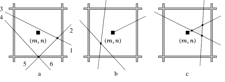
1 2 3

4

5 6

(

m;n

) (

m;n

) (

m;n

)

[image:16.612.105.489.110.250.2]

a b c

Figure 5: Vertex (

m;n

) and chord ordering.

To limit this number, the chord endpoints of the exact polylines are rounded to odd integer values. Chord intersection is done on the rounded chords and the intersection points are exactly represented as rational numbers. To use an existing intersection point as the endpoint of a new curve without increasing the bit length, we consider the semi-open rectangles

R

m;n

= [

m

1

;m

+ 1)[

n

1

;n

+ 1), where

m

and

n

are odd. Since the vertical and horizontal lines limiting the rectangles have even coordinates, there are no rounded chords collinear with these lines. So, it is always possible, if two or more chords intersect inside

R

m;n

, to order them along the boundary of

R

m;n

by using either the coordinates of their intersections with the lines limiting the rectangle or their slopes if they leave

R

m;n

at exactly the same point (Fig. 5a). We define the center of

R

m;n

as the vertex of the intersection points lying inside

R

m;n

. This associates intersection points with vertices but does not round their coordinates. To use a chord intersection point as the endpoint of a new curve, we do not use the point itself but its vertex (Fig. 5b). Therefore, small faces lying inside a single rectangle will not be represented in the map data structure (Fig. 5c).

On a polycurve, an intersection point is represented as a parameter value

p

= (

i;u

) where

i

is the chord index on the polyline and

u

is a rational number giving the exact position of the point on the chord. Since all chords have now rounded endpoints, ordering two intersection points along one curve requires at most 4

b

+ 6 bits. It is possible to reduce this bound by further subdividing the chords, using a larger value of

k

which can be deduced from equation (7). However, this implies also subdividing the line segments which may be part of a polycurve.

We also need to order the intersections of the chords with the lines limiting the rectangles

above, the intersection algorithm uses this information to return only actual intersections. A polycurve is removed from the map data structure iff it has been totally erased.

This method has two limitations. First, intersection is performed on the rounded polylines. Thus, there are situations (e.g. tangencies) where intersections between the true polycurves are ignored. Likewise, polylines may intersect even if true polycurves do not (e.g. two concentric circles with very close radii interpolated by regular polygons whose sides intersect pairwise). Second, the topology of a map computed in this way is not invariant under a general affine transform. Thus, the map has to be recomputed from the original data whenever it is rotated or scaled. The first limitation is inherent in any linear interpolation process. However, for 2D graphics applications, it is always possible to prevent any visible effects by choosing an appropriate grid size. The second limitation can only be solved by using exact arithmetic on real numbers or symbolic computation on algebraic curves, which are currently too slow for interactive applications. Without recomputing the map, it is possible to perform integer translation (e.g. when dragging a map) if we remain inside the grid.

In this section, we have shown that a robust method for the computation of planar maps with linearly interpolated B´ezier curves requires at most

b

+ (

k

+ 1)

d

bits for the forward differencing step and 4

b

+ 6 bits for the intersection and sorting steps. Our implementation uses an efficient arbitrary precision integer arithmetic package coded in assembly language [24]. In practice, the average size of the numbers involved in the process is much smaller than the above bounds. The only operation we must perform on rational numbers is comparison, which is two integer multiplications and a test. This operation can be optimized by computing and comparing the two cross products digits in high to low order. The value of

b

is a parameter of the program, allowing the grid size to be adapted to the resolution of the display.

4 Data Structure and Algorithms

After describing the planar map data structure, we detail below the two main algorithms. Curve insertion uses point location in a map to find the face containing the first endpoint of a polycurve, but we first describe insertion since point location is performed as the insertion in the map of a dummy line segment.

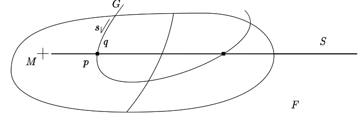
4.1 Planar Map Description

A map contains two different sets of data. The first one describes the geometry of the polycurves and their intersections, and the second contains the topological data. In what follows, the word polycurve should be understood as the rounded polyline associated with the polycurve.

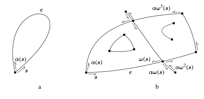
s

(

s

)

e

s

(

s

)

!

(

s

)

!

(

s

)

!

2₍

s

₎

!

5₍

s

₎

e

[image:18.612.110.460.86.257.2]

a b

Figure 6: Map topology.

as in Sec. 3.4. In the transverse case, an intersection yields two points, one on each polycurve. As parameters are totally ordered along a polycurve, an arc is noted below as a parameter interval [

p

1

;p

2]. Arcs are marked as either erased or non-erased.

Topology. The mapping defined in Sec. 3.4 associates with each point a unique vertex. To support arc overlap, we attach to an arc an edge connecting its vertices. Arcs lying entirely in one rectangle

R

m;n

are not considered. Overlapping arcs share the same edge. The geometry of an edge is the geometry of one of the arcs it supports. Different edges can connect the same pair of vertices. The ordering of the edges around a vertex is the chord ordering defined by the rectangles

R

m;n

.

To access the faces of a planar map, it is convenient to consider an edge as two directed edges, called sides. If an edge

e

is a loop incident to the vertex

v

, then the clockwise (cw) and counterclockwise (ccw) orientations along

e

define the two sides associated with

e

(Fig. 6a). Two mappings are defined on the sides of a map:

(

s

) is the side next to

s

in the ccw order around the vertex incident to

s

, and

!

(

s

) is the other side of the edge [17]. We note the ordering of the sides around a vertex,

-order. To follow the boundary containing a side

s

, the compound mapping

!

is applied repeatedly until back in

s

(Fig. 6b). The result is a face boundary called a contour. Contours with a ccw orientation are outer contours, others are inner contours. Adding a virtual inner contour located at infinity, there is exactly one inner contour for each face of a map.

4.2 Polycurve Insertion

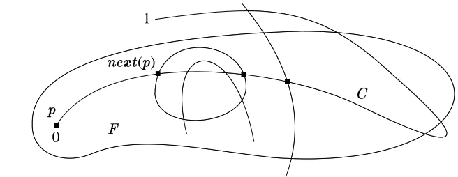
A non–erased arc is visible in a face if it is supported by an edge of which at least one side is in a contour bounding the face. Polycurve insertion uses the method described in Sec. 3 to compute the intersections between a new polycurve

C

and all the arcs visible in the faces where

C

is lying (Fig. 7). Along

C

,

p

is the current parameter value and

next

(

p

) is either 1 or the parameter value of the next intersection point,

p < next

(

p

).

0

F

p

next

(

p

)

C

[image:19.612.93.421.195.322.2]

1

Figure 7: Polycurve insertion (first iteration).

Step 1. Using point location (Sec. 4.4), find the face

F

containing the first point of

C

. Set parameter

p

to 0.

Step 2. If

F

has already been processed, jump to step 3. Otherwise, compute the intersections between arc [

p;

1] and all the arcs visible in

F

. Cut the arc [

p;

1] and the intersected arcs of

F

at each intersection point and create the corresponding vertices and sides. At the end of this step, there are no more intersections between

p

and

next

(

p

), and the

-order around the vertices along

C

has been updated.

Step 3. If there is no overlapping, create an edge between the vertices associated with

p

and

next

(

p

), link it with the arc [

p;next

(

p

)] in the data structure, and update the inclusion tree accordingly (see section 4.3). Otherwise, the edge already exists, so link it with the arc [

p;next

(

p

)].

Step 4. If

next

(

p

) = 1 then stop. Otherwise, let

s

be the side of arc [

next

(

p

)

; next

(

next

(

p

))] associated with

next

(

p

). Since the

-order around the two corresponding points is known,

s

is known. Set

F

to the face incident to

(

s

), and

p

to

next

(

p

). Repeat step 2.

An arc is visible in at most two faces but an existing polycurve

G

can be visited several times. However, the intersection between the arc [

p;

1] of

C

and

G

is done only once: the first time an arc of

G

becomes visible in the current face

F

. The intersection points located outside

4.3 Updating the Inclusion Tree

The insertion algorithm uses the contour inclusion tree to find all visible arcs in a face. Contours are modified by edge addition and edge removal. This section details the operations on the inclusion tree. We begin by edge classification.

The degree

d

of a vertex

v

is the number of sides incident to

v

, and

v

is a dangling vertex if

d

(

v

) = 1. If both sides of an edge are in the same contour, it is a dangling edge, otherwise it is a border edge. A dangling edge is connecting if it has no dangling vertex, terminal if it has exactly one dangling vertex, and isolated if it has two dangling vertices. A loop incident to a vertex

v

with

d

(

v

) = 2 is an isolated border edge.

An edge falls into one of the following types:

1. a terminal edge with both sides in an inner contour,

2. a connecting edge with both sides in an inner contour,

3. a border edge with both sides in two distinct inner contours,

4. a border edge with one side in an inner contour and the other side in an outer contour,

5. an isolated edge,

6. a terminal edge with both sides in an outer contour,

7. a connecting edge with both sides in an outer contour,

8. an isolated border edge.

When inserting a polycurve, new edges may be added to the map. Adding an edge implies creating its sides, vertices, and updating the

-order around the vertices. The updated contours are thus available through the mapping

!

. The inclusion tree is updated after each edge addition, so it is therefore possible to find the type of a new edge by counting its dangling vertices and checking the updated contours. The inclusion tree is then updated by performing the following actions, indexed by edge type:

2. merge: inner&outer!inner,

3. split: inner!inner&inner,

4. split: outer!outer&inner,

5. create: outer,

7. merge: outer&outer!outer,

For example, if an edge of type 2 is added to a map, one inner contour and one outer contour are merged to give a single inner contour.

When erasing a polycurve or an arc, existing edges may be removed from the map. The inclusion tree is updated before each existing edge removal, using the same tests as above. When the type of the edge has been found, the inclusion tree is updated by performing the following actions, indexed by edge type:

2. split: inner!inner&outer,

3. merge: inner&inner!inner,

4. merge: outer&inner!outer,

5. delete: outer,

7. split: outer!outer&outer,

8. delete: outer&inner.

Adding or removing an edge of type 1 or 6 (i.e., terminal edges) does not modify the inclusion tree.

4.4 Point Location

Given a query point with integer coordinates, the point location algorithm returns either a face, an edge, or a vertex. In map sketching, all selections are done through this algorithm (e.g. coloring a face or selecting an existing intersection as the endpoint of a new polycurve). One method is to intersect a line segment

S

with all polycurves.

S

is defined by the query point

M

, with parameter 0, and a point outside the bounding box of the map, with parameter 1. If no intersection is found,

M

is inside the infinite face. Else, retain the polycurve

G

whose intersection is closest to

M

. This intersection is known by its parameter values

p

on

S

and

q

on

G

. The parameter

q

gives the arc of

G

containing the intersection. If

p

= 0, then

M

is exactly on the edge supporting this arc. Otherwise,

M

is inside one of the two faces incident to the edge. The side which sees

M

to its right gives the answer (a side defines a unique orientation on a polycurve).

This method does not take advantage of the partition of the plane defined by the faces of the map. To reduce the average number of visited polycurves, the following algorithm uses face adjacency (Fig. 8). This algorithm is similar to the polycurve insertion algorithm, but it uses polycurve intersection instead of arc intersection. A polycurve is visible in a face if one of its non–erased arcs is visible in the face.

M

s

q

p

G

[image:22.612.125.481.96.212.2]

F

S

Figure 8: Point location.

Step 2. If

F

has no outer contours then return

F

. Otherwise, intersect

S

with the polycurves visible in the outer contours of

F

(if two or more polycurves are overlapping, it is enough to consider one of them). If there is no intersection, return

F

. Otherwise, let

e

be the edge which gives the smallest parameter

p

on

S

, and

s

the side of

e

which sees

M

to its right. If

s

is part of an outer contour, return

F

. Otherwise, set

S

to [0

;p

] and set

F

to the face incident to

s

.

Step 3. Intersect

S

with the polycurves visible in the inner contour of

F

. If there is no intersection, call recursively step 2. Otherwise, let

e

be the edge which gives the smallest parameter

p

on

S

, and

s

the side of

e

which sees

M

to its right;

s

is necessarily part of an inner contour. Set

F

to the face incident to this contour and

S

to [0

;p

]. Repeat step 3.

Like polycurve insertion, point location may visit a polycurve several times, but only one intersection with

S

is performed. The geometric tests are performed on rational numbers, thus they are exact. Indications on the complexity of both algorithms are given by the horizon theorem for Jordan curves included in [8]. However, this last result cannot be applied in a straightforward way as the number of intersections between two polylines may be greater than the number of intersections between the true polycurves, and the polylines may be partially overlapping.

5 Conclusion

[image:23.612.71.511.164.710.2]

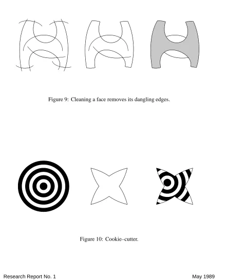
Though it has some limitations, the method described in this report provides a powerful tool for constructing illustrations. The planar map data structure and algorithms also allow for automated compound operations, such as the ones described in Fig. 9 and Fig. 10. Fig. 11 and 12 show illustrations produced with the map sketching technique.

[image:23.612.90.463.177.307.2]

Figure 9: Cleaning a face removes its dangling edges.

[image:24.612.126.463.137.480.2]

[image:25.612.70.508.85.540.2]

References

1. Baroni, D. Art Graphique Design. Editions du Chˆene, Paris (1987).

2. Baudelaire, P. and Gangnet, M. Planar Maps: an Interaction Paradigm for Graphic Design. In CHI’89 Proceedings, Addison-Wesley (1989).

3. Bentley, J.L. and Ottmann, T.A. Algorithms for Reporting and Counting Geometric Intersections. IEEE Trans. on Comput., 28, 9 (1979).

4. DeRose, T.D. and Barsky, B.A. Geometric Continuity for Catmull-Rom Splines. ACM Transactions on Graphics, 7, 1 (1988).

5. Dobkin, D. and Silver, D. Recipes for Geometry and Numerical Analysis. In Proceedings of the Fourth Annual ACM Symposium on Computational Geometry, ACM Press, New York (1988).

6. Edelsbrunner, H. Algorithms in Combinatorial Geometry. Springer-Verlag, New York (1987).

7. Edelsbrunner, H. and Guibas, L.J. Topologically Sweeping an Arrangement. Research Report #9, Digital Equipment Systems Research Center, Palo Alto (1986).

8. Edelsbrunner, H., Guibas, L., Pach, J., Pollack, R., Seidel, R., and Sharir, M. Arrangements of Curves in the Plane: Topology, Combinatorics, and Algorithms. In Fifteenth ICALP Coll. (1988) 214–229.

9. Forrest, A. R. Geometric Computing Environments: Some Tentative Thoughts. In Theoretical Foundations of Computer Graphics and CAD, Springer-Verlag (1988).

10. Gangnet, M. and Herv´e, J.C. D2: un ´editeur graphique interactif. In Actes des Journ´ees SM90, Eyrolles, Paris (1985).

11. Greene, D.H. and Yao, F.F. Finite–Resolution Computational Geometry. In Proc. 27th IEEE Symp. on Found. Comp. Sci., Toronto (1986).

12. Guibas, L. and Stolfi, J. Primitives for the Manipulation of General Subdivisions and the Computation of Voronoi Diagrams. ACM Transactions on Graphics, 4, 2 (1985).

13. Hoffmann, C.M., Hopcroft, J.E., and Karasick, M.S. Towards Implementing Robust Geometric Computations. In Proceedings of the Fourth Annual ACM Symposium on Computational Geometry, ACM Press, New York (1988).

15. Lane, J.F. Curve and Surface Display Techniques. Tutorial, ACM SIGGRAPH’81 (1981).

16. Lien, S.L., Shantz, M., and Pratt, V. Adaptive Forward Differencing for Rendering Curves and Surfaces. ACM Computer Graphics, Vol. 21, 4 (1987) 111–118.

17. Lienhardt, P. Extensions of the Notion of Map and Subdivision of a Three–Dimensional Space. In STACS’88, Lecture Notes in Computer Science 294 (1988).

18. Michelucci, D. Th`ese. Ecole Nationale Sup´erieure des Mines de Etienne, Saint-Etienne (1987).

19. Michelucci, D. and Gangnet, M. Saisie de plans `a partir de trac´es `a main-lev´ee. In Actes de MICAD 84, Herm`es, Paris (1984).

20. Preparata, F.P. and Shamos, M.I. Computational Geometry: an Introduction. Springer-Verlag, New York (1985).

21. Ramshaw, L. Blossoming: A Connect-the-Dots Approach to Splines. Research Report #19, Digital Equipment Systems Research Center, Palo Alto (1987).

22. Schultz, M. H. Spline Analysis. Prentice Hall (1973).

23. Sederberg, T.W. and Parry, S.R. Comparison of three curve intersection algorithms. Computer-Aided Design, Vol. 18 (1986).

24. Serpette, B., Vuillemin, J., and Herv´e, J.C. BigNum: a Portable and Efficient Package for Arbitrary Precision Arithmetic. Research Report #2, Digital Equipment Paris Research Laboratory, Rueil-Malmaison (1989).

25. Tutte, W.T. Graph Theory. Addison-Wesley (1984).

The following documents may be ordered by regular mail from:

Librarian – Research Reports Digital Equipment Corporation Paris Research Laboratory 85, avenue Victor Hugo 92563 Rueil-Malmaison Cedex France.

It is also possible to obtain them by electronic mail. For more information, send a message whose subject line [email protected], from within Digital, todecprl::doc-server.

Research Report 1: Incremental Computation of Planar Maps. Michel Gangnet, Jean-Claude Herv ´e, Thierry Pudet, and Jean-Manuel Van Thong. May 1989.

Research Report 2: BigNum: A Portable and Efficient Package for Arbitrary-Precision Arithmetic. Bernard Serpette, Jean Vuillemin, and Jean-Claude Herv´e. May 1989.

Research Report 3: Introduction to Programmable Active Memories. Patrice Bertin, Didier Roncin, and Jean Vuillemin. June 1989.

Research Report 4: Compiling Pattern Matching by Term Decomposition. Laurence Puel and Asc ´ander Su ´arez. January 1990.

Research Report 5: The WAM: A (Real) Tutorial. Hassan A¨ıt-Kaci. January 1990.

Research Report 6: Binary Periodic Synchronizing Sequences. Marcin Skubiszewski. May 1991.

Research Report 7: The Siphon: Managing Distant Replicated Repositories. Francis J. Prusker and Edward P. Wobber. May 1991.

Research Report 8: Constructive Logics. Part I: A Tutorial on Proof Systems and Typed

-Calculi. Jean Gallier. May 1991.

Research Report 9: Constructive Logics. Part II: Linear Logic and Proof Nets. Jean Gallier. May 1991.

Research Report 10: Pattern Matching in Order-Sorted Languages. Delia Kesner. May 1991.

Research Report 13: Functions as Passive Constraints in LIFE. Hassan A¨ıt-Kaci and Andreas Podelski. June 1991.

Research Report 14: Automatic Motion Planning for Complex Articulated Bodies. J ´er ˆome Barraquand. June 1991.