Hydrol. Earth Syst. Sci., 18, 1857–1872, 2014 www.hydrol-earth-syst-sci.net/18/1857/2014/ doi:10.5194/hess-18-1857-2014
© Author(s) 2014. CC Attribution 3.0 License.
Determination of cost coefficients of a priority-based water
allocation linear programming model – a network flow approach
F. N.-F. Chou and C.-W. Wu
Department of Hydraulic and Ocean Engineering, National Cheng Kung University, 1 University Rd., Tainan, Taiwan
Correspondence to: C.-W. Wu ([email protected])
Received: 6 November 2013 – Published in Hydrol. Earth Syst. Sci. Discuss.: 10 December 2013 Revised: – – Accepted: 28 March 2014 – Published: 21 May 2014
Abstract. This paper presents a method to establish the ob-jective function of a network flow programming model for simulating river–reservoir system operations and associated water allocation, with an emphasis on situations when the links other than demand or storage have to be assigned with nonzero cost coefficients. The method preserves the priori-ties defined by rule curves of reservoir, operational prefer-ences for conveying water, allocation of storage among mul-tiple reservoirs, and transbasin water diversions. Path enu-meration analysis transforms these water allocation rules into linear constraints that can be solved to determine link cost coefficients. An approach to prune the original system into a reduced network is proposed to establish the precise con-straints of nonzero cost coefficients, which can then be effi-ciently solved. The cost coefficients for the water allocation in the Feitsui and Shihmen reservoirs’ joint operating system of northern Taiwan was adequately assigned by the proposed method. This case study demonstrates how practitioners can correctly utilize network-flow-based models to allocate water supply throughout complex systems that are subject to strict operating rules.
1 Introduction
The allocation of water in river–reservoir systems usually involves a number of priority-based decisions, which in-clude water rights, reservoir operating rules, commitments and negotiation between stakeholders, preferences for the conveyance of water and other requirements. Such systems usually comprise reservoirs, weirs, river channels, canals, di-version tunnels, pipelines and treatment plants as well as the demands of different purposes. The configuration of a
regional system may extend to include multiple reservoirs, transbasin diversion and in-stream flow requirements at dif-ferent reaches. Such modeling is further complicated by the need to determine the ideal means of regulating flow, such that demands are satisfied according to assigned priorities, while minimizing the residual water flowing into the receiv-ing water body to ensure the efficient utilization of water re-sources. The means by which water is moved must also con-form to the associated conveyance capacity.
1858 F. N.-F. Chou and C.-W. Wu: Priority-based water allocation linear programming model that “the results from the system analysis tool are not
eas-ily understood by the stakeholders, and government repre-sentatives of different countries bear some suspicion about the results”. In order to resolve this problem, two other nonoptimization-based models were evaluated and compared with the original one. Nevertheless, the authors still could not conclude on which model was more adequate for their case due to the structurally differences of simulating water alloca-tion priorities in different models.
As a specialization of LP, network flow programming (NFP) only focuses on solving a specific subset of general LP problems that can be formulated in a more restrictive format. This loss of generality allows the resources alloca-tion problem to be visually and precisely displayed by the network structure, and gains in return higher computational efficiency and easier comprehension of the priority-based allocation mechanism. These characteristics have prompted model developers to incorporate NFP into many general models (Evenson and Moseley, 1970; Sigvaldason, 1976; Labadie et al., 1986; Martin, 1987; Kuczera and Diment, 1988; Brendecke, 1989; Chung et al., 1989; Andrews et al., 1992; Wurbs, 1993; Andreu et al., 1996; Yerrameddy and Wurbs, 1996; Fredericks et al., 1998; Ilich et al., 2000; Dai and Labadie, 2001; Chou and Wu, 2010). The NFP represents the physical aspect of a water resources system as a directed networkG(N,L), whereN is the set ofnnodes andLis the set ofmlinks. The formulation of a minimum cost NFP problem can be expressed as (Ahuja et al., 1993)
minimize P (i,j )∈L
cij·xij (1)
subject to X
{j:(i,j )∈L}
xij− X
{j:(j,i)∈L}
xj i=0 for alli∈N (2)
lij≤xij ≤uijfor all(i, j )∈L, (3) whereiandj are the indices of node; (i,j )is the link from the tail nodeito the head nodej;xij represents the amount of flow on link (i,j );cij is the unit shipping cost along link (i,j );lij anduij are the lower and upper limits on flow in link (i,j ).
In a NFP-based water allocation model, nodes can rep-resent storage or nonstorage points of confluence or diver-gence, and links represent reservoir outlet works, channels or pipes, water consumption, and carryover storage. Equa-tion (2) indicates the continuity and availability of water at a node, for it states that the flow out of the node should equal to all incoming water. The upper and lower limits of a link represent its physical flow capacity, thus Eq. (3) states the transportability of water conveyance. The cost coefficient promotes flow routes that minimize net cost, thus determin-ing the most preferable allocation of water supply with re-spect to a given allocating rule. Thus, correct assignment of link cost coefficients to reflect respective priorities is a neces-sary condition for any effective applications of not only NFP
but LP-based water allocation models. Most common appli-cations directly assign the cost coefficients related to the links of carryover storage or water consumption to represent the priorities of associated stakeholders. However, there are situ-ations when internal links other than demand or storage have to be assigned with nonzero costs in order to achieve spe-cific allocation requirements, such as water conveyance pref-erence or surplus water diversion. This type of assignment is not straightforward for practitioners with little theoretical background, especially when forced to deal with a regional system of multiple reservoirs, water conveyance routes, in-stream flow requirements and transbasin water diversions.
The concept of developing a method for establishing cost coefficients of NFP models to adequately represent water allocation priorities was originally proposed by Israel and Lund (1999). Ferreira (2007) further broadened the scope for more general LP problems by demonstrating how different types of side constraints and variables in the LP formulation may affect the priorities defined by the cost coefficients of links in the NFP subset. These previous works represented the priority requirement as a set of rules. The rules were com-piled into an LP problem that is solved as a means of initializ-ing the actual allocation model (Ferreira, 2007). The present study follows and expands upon this principle with the pro-posal of additional allocation rules and a path-enumeration algorithm to facilitate automation of the cost-determination procedure. The presented rules allow one to simulate such water allocation priorities as reservoir rule curves, storage allocation among multiple reservoirs, preferred water mains, and transbasin diversion of surplus water. Path enumeration analysis is adopted to convert user-specified water supply al-location rules into a set of constraints; solving these con-straints yields the cost coefficients that adhere to all speci-fied rules. Further, an approach to prune the original system into a reduced network is proposed to establish the precise constraints of nonzero cost coefficients, which can then be efficiently solved. This pruned procedure thus functions suc-cessfully to efficiently initialize an effective application of water allocation models.
2 Water allocation model
2.1 Alternative approaches: linear programming vs. network flow programming
The following presentation of methodology uses a NFP framework to demonstrate the procedure of determining cost coefficients. This concept is helpful to interpret the establish-ment of an objective function for more generalized LP-based models. One of the major differences between these alter-native optimization approaches in modeling water resources allocations is how the non-NFP constraints, which cannot be represented by Eqs. (2) and (3), are incorporated. These con-straints usually originate from the need to simulate physical
F. N.-F. Chou and C.-W. Wu: Priority-based water allocation linear programming model 1859 water movement processes, such as return flows, flow losses,
reservoir evaporation, and channel routing effects. In pure NFP-based models, these features have been handled through the use of successive iterations (Ilich, 2008, 2009). These it-erative processes are external to the algorithmic solving pro-cedure. Usually the lower or upper limits of links are itera-tively adjusted to meet non-NFP constraints; thus, the prior-ities specified by link costs are unchanged during iterations. By contrast, an LP solver can directly incorporate non-NFP features into the formulation and the algorithmic solving pro-cedure. However, this flexibility may impair the character-istic of priority-based water allocation of NFP. One simple example is that water may be allocated to a junior-priority demand with less flow loss, rather than a senior demand with greater flow loss, if the objective function is not appropri-ately set up in the LP formulation. Another example is the effect of channel flow routing, which may be easily mod-eled by the Muskingum method and incorporated into an LP formulation. Suppose that there are two demands located at the upstream and downstream ends of a river channel, re-spectively, with junior and senior priorities. The travel time required for water to flow through the channel from the loca-tion of upstream (junior) demand to downstream (senior) de-mand exceeds the unit time period of an LP-based simulation model. The portion of water that does not reach the point of downstream demand cannot explicitly contribute to the ob-jective function in the current unit time period. The solution to this issue, similar to that for the flow loss case, consists of allocating water to the junior demand first instead of maxi-mizing satisfaction of the senior downstream demand, if the discrepancy between their assigned cost coefficients is not large enough to compensate for the retained and ineffective portion of water.
While NFP-based models are still widely utilized, several general software packages have updated their optimization engines with LP solvers to manage the rising demand for simulating non-NFP constraints and variables. Some exam-ples include CALSIM (Draper et al. 2004), OASIS (Hydro-logics, Inc., 2009) and WEAP (Stockholm Environment In-stitute, 2011). Nonetheless, the impacts of non-NFP features on water allocation have not been adequately discussed; only Israel and Lund (1999), Labadie and Baldo (2001), and Fer-reira (2007) have addressed this topic. Since non-NFP con-straints must be strictly satisfied, they could be regarded as a higher level of priorities that would supersede and may disturb the priorities originally defined in the NFP subset as stated by Ferreira (2007). A desired resolution may be to achieve a simultaneous satisfaction of these two levels of priorities, if such a condition is feasible. In order to achieve this goal, the impact of non-NFP features on the allocation mechanism must be explicitly incorporated into the cost-determining procedure. Such as the two non-NFP constraints mentioned above, water transmission loss and flow routing can be modeled as the portion of water that is lost or de-layed while allocating water to senior demands. This
por-tion of water is ineffective to the objective funcpor-tion; the as-signed link costs should be able to withstand these impacts to preserve the priorities of water allocation. For practical purposes, however, the present study focuses solely on de-termination of link costs for NFP-based modeling. Future re-search may extend to derive a comprehensive approach for more generalized LP-based models, thus accounting for all types of non-NFP constraints that may be encountered in real-world applications.
2.2 Framework of a network flow programming-based allocation model
NFP-based water allocation models can be used to allocate water over single or multiple time steps. For models that allo-cate water across multiple time steps, links connect reservoir nodes in different time periods to represent carryover storage. These models have been applied in reservoir sizing (Kuczera, 1989; Khaliquzzaman and Chander, 1997), capacity expan-sion (Martin, 1987; Gondolfi et al., 1997), the derivation of reservoir operating rules (Lund and Ferreira, 1996; Bessler et al., 2003), water transfer during droughts (Cheng et al., 2009), and the optimal real-time flood control operation of reservoirs (Braga and Barbosa, 2001). Single time step mod-els allocate water only within an operational unit period, but the allocation is sequentially solved in every step during the simulation time horizon. Routing results produced in this manner are useful for quantifying the expected water supply situation and the risks of water shortage under the simulated conditions. This study discusses the assignment of cost coef-ficients for the single time step model.
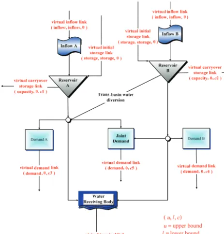
Figure 1 illustrates a water resources system as a network during a unit operational period. Virtual links illustrated by dotted lines satisfy Eq. (2), which specifies continuity equa-tions of nodes, by conveying water into and out of the sys-tem. These virtual links signify the inflow of system, initial and carryover storage of reservoir, water consumed by the stakeholders, and the water body that receives surplus flow. 2.3 Principle in assigning cost coefficients and the
necessity of preprocessing analysis
1860 F. N.-F. Chou and C.-W. Wu: Priority-based water allocation linear programming model
11
201
Fig. 1. Network structure of water resources system 202
203
2.3 Principle in assigning cost coefficients and the necessity of preprocessing 204
analysis 205
The cost coefficients of links, generalized by Fig. 1, quantify the relative priority 206
of each respective water user. These cost coefficients must reflect the flow priorities 207
[image:4.612.50.282.67.309.2]associated with demand or storage under predefined operating conditions. One 208
Figure 1. Network structure of water resources system.
enough to achieve the allocation requirements. One simple example is that minor costs such as−1 or+1 are commonly assigned on links where flow is to be encouraged, such as hydropower plant, or discouraged, such as routes with high transmission loss.
Another example is the transbasin diversion of surplus wa-ter, which requires diverting the required surplus water of a system into the adjacent system to enhance the efficiency of water utilization. An intuitive way to achieve this require-ment is to use the iterative approach suggested by Labadie and Baldo (2001). This approach recommends a conceptual “flow-through” demand to be placed in the transbasin tun-nel. This demand is given a lower priority than all demands or storage in the system to be diverted, which guarantees that transbasin diversions only occur once all demands in the original system are satisfied. According to the water supplied to the flow-through demand, iterations are then performed to artificially inject this diverted water into the adjacent system. Thus, transbasin diversion will work as long as the original system has surplus water, regardless of the hydrological con-dition of the other system. However, there is no need to per-form diversion when both systems are in abundance of water, for the diverted flow will become surplus to the other system. Although the “flow-through” approach is capable of simulat-ing physical water movement process such as nonconsump-tive water usage, it may not properly model the operational features, such as adequate timing of diversion in this situa-tion. This is especially critical when the transbasin diversion is charged with money; thus, unnecessary diversions should be avoided. Inevitably, satisfying the condition of surplus
wa-14
two rules are more elaborated in this paper, with two additional rules, trans-basin surplus 253
diversion and water conveyance preference, being proposed to constitute the 254
comprehensive analyzing framework as shown in Fig. 2. Water allocation rules and cost-255
determining procedure is described in detail in the following section. 256
257
258
Fig. 2 Cost determining procedure proposed in this study
259
260
3 Water Allocation Rules
261
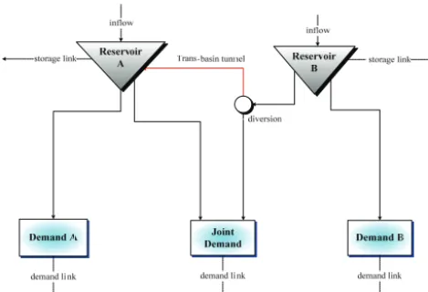
3.1 Rule 1: Trans-basin diversion of surplus water
262
Generally, the development of a new trans-basin water diversion project must not 263
impact existing users of the system. Fig. 3 depicts a simple example, in which only 264
surplus water in the system associated with reservoir B can be diverted for storage in 265
reservoir A. Thus, the first rule allows users to specify a link in the network representing 266
Figure 2. Cost determining procedure proposed in this study.
ter diversion requires assigning a positive cost on the link of the transbasin tunnel, without using the flow through demand approach.
The determination of cost becomes more complicated if a combination of various allocation rules is involved, such as different operating rule curves for individual reservoirs, preferences of water conveyances in multiple locations, the allocation of multireservoir storage, and transbasin water di-versions. When multiple links in the system have to be as-signed with nonzero cost coefficients, the accumulation of costs along a flow path to a demand/reservoir might impair its priority, which is originally dictated by the cost of the vir-tual link. The connectivity between links of nonzero costs has to be identified to ensure that the sum of cost coefficients in paths to a water usage of higher priority is always less than the total costs of any path to a lower priority stakeholder. If the user cannot ensure assigning nonzero costs on the links to achieve the allocation requirements, a general preprocessing analysis will have to assume that the cost coefficient of every link in the system is unknown.
This study develops a procedure to establish the objective function of NFP-based water allocation models, in which all representative allocation rules encountered are considered. The allocation associated with reservoir operating rule curves and multireservoir storage balancing was preliminarily ad-dressed in Chou and Wu (2011). These two rules are more elaborated in this paper, with two additional rules, transbasin surplus diversion and water conveyance preference, being proposed to constitute the comprehensive analyzing frame-work as shown in Fig. 2. The water allocation rules and cost-determining procedure are described in detail in the follow-ing section.
[image:4.612.310.543.70.243.2]F. N.-F. Chou and C.-W. Wu: Priority-based water allocation linear programming model 1861
15
a way of distributing water with last priority. The priorities of all paths through this 267
specific link are junior to any other paths to demands and storage in the system. 268
269
270
Fig. 3 Example of trans-basin water diversion 271
272
Let L be the set of all links, LD be the set of virtual demand links, LS be the set of 273
virtual storage links in the network, and (LD + LS)be the union of LD and LS. Define a 274
path as a sequence of links without the repetition of head nodes, i.e., with no cycle in the 275
path. Use RLP to represent the set of paths containing the specific link for the diversion
276
[image:5.612.50.285.66.226.2]of surplus water, and RLD+LS to represent the set of paths with the final links belong to 277
Figure 3. Example of transbasin water diversion.
3 Water allocation rules
3.1 Rule 1: transbasin diversion of surplus water Generally, the development of a new transbasin water diver-sion project must not impact existing users of the system. Figure 3 depicts a simple example in which only surplus wa-ter in the system associated with reservoir B can be diverted for storage in reservoir A. Thus, the first rule allows users to specify a link in the network representing a way of distribut-ing water with last priority. The priorities of all paths through this specific link are junior to any other paths to demands and storage in the system.
LetLbe the set of all links,LDbe the set of virtual
de-mand links,LSbe the set of virtual storage links in the
net-work, and (LD+LS)be the union ofLD andLS. Define a
path as a sequence of links without the repetition of head nodes, i.e., with no cycle in the path. UseRLP to represent
the set of paths containing the specific link for the diversion of surplus water, and RLD+LS to represent the set of paths
with the final links belonging to (LD+LS). The
mathemati-cal formulation of priority requirement for surplus water di-version can be expressed as
max[cost(RLD+LS−RLP)]<min[cost(RLP)], (4)
where(RLD+LS−RLP)is the same asRLD+LSbut excluding
RLP, cost is a function used to calculate the sum of the cost
coefficients of the links in a path, and cost (RLP)represents
the set of total costs for all paths inRLP. Equation (4) states
that the largest cost conducted by paths that do not pass from the transbasin link is less than the lowest cost by passing from the transbasin link. Because the lowest priority should corre-spond to the largest cost under the framework of NFP, a set of cost coefficients that satisfies this condition should guarantee that the transbasin link will work only in case of surplus.
For a total of np1apaths inRLPwhere thekth path is
rep-resented asP1ak, a Kronecker delta function can be used to
represent ifP1akcontains link (i,j ):
∀(i, j )∈L, δ1a(i,j )k =
1 if(i, j )∈P1ak
0 otherwise . (5)
Suppose that(RLD+LS−RLP)contains np1blinks andP1bk
represents thekth path in(RLD+LS−RLP). Another
Kro-necker deltaδ1b(i,j )k can be used to represent ifP1bkcontains link (i,j ):
∀(i, j )∈L, δ1b(i,j )k =
1 if(i, j )∈P1bk
0 otherwise . (6)
Equation (4) can then be expressed by the following con-straints:
X (i,j )∈L
δ1a(i,j )k c(i,j )≥CMin1 k=1, ...,np1a, (7)
X (i,j )∈L
δ1b(i,j )k c(i,j )≤CMax1 k=1, ...,np1b, (8)
CMax1+ε≤CMin1, (9)
wherec(i,j )is the cost coefficient per unit flow of link (i,j ), CMin1represents the lower bound of the total costs of paths
inRLP,CMax1 represents the upper bound of the total costs
of paths in(RLD+LS−RLP), and εis an arbitrary positive
integer specified by the user.
3.2 Rule 2: priorities between water usages and reservoir storage
The basic framework of water allocation in the water re-sources system is the priorities between water usages and reservoir storage. The priorities may be defined by water rights, judicial or legislative actions to protect specific wa-ter usages, private agreements between stakeholders or the operating rule curves of reservoirs. Chou and Wu (2011) il-lustrated the setting of priorities between demands and stor-age for the operating rule curves commonly adopted in indi-vidual reservoir operating systems of Taiwan. The proposed mathematical formulation was as follows.
Assume that (LD+LS) is the set that consists of all
vir-tual demand and storage links. (LD+LS) (k)is the link pri-oritizedkth among (LD+LS). Equation (10) prioritizes all
virtual demand and storage links that comprise a water sup-ply network as follows:
max{cost[RLD+LS(k)−RLP]}< (10)
min{cost[RLD+LS(k+1)−RLP]}, k=1∼md+ms−1.
In Eq. (10), the setRLD+LS(k)consists of all potential flow
routes with final link asLD+LS(k),RLPis the same as
de-fined in Eq. (4) of Sect. 3.1; andmd+msrepresents the
num-ber of links in (LD+LS). Equation (10) states that the largest
1862 F. N.-F. Chou and C.-W. Wu: Priority-based water allocation linear programming model The following constraints can be established from the
con-cept of Eq. (10), derived by a similar process of converting Eq. (4) into Eqs. (7)–(9) as shown in Sect. 3.1.
CMin2k ≤
X (i,j )∈L
δ2(i,j )k,l c(i,j )≤CMax2k l=1, ..,np2,k,
k=1, ..., md+ms, (11)
CMax2k+ε≤CMin2k+1 k=1, ..., md+ms−1, (12)
where CMax2k and CMin2k define the feasible range of net
conveyance costs for flow paths in RLD+LS(k)−RLP; the
Kronecker delta functionδ2(i,j )k,l indicates whether thelth flow path ofRLD+LS(k)−RLPincludes the link(i, j ), np2,kis the
number of paths that exist inRLD+LS(k)−RLP, andεis the
same as in Eq. (9), which is used to maintain an interval of costs between consecutive priorities.
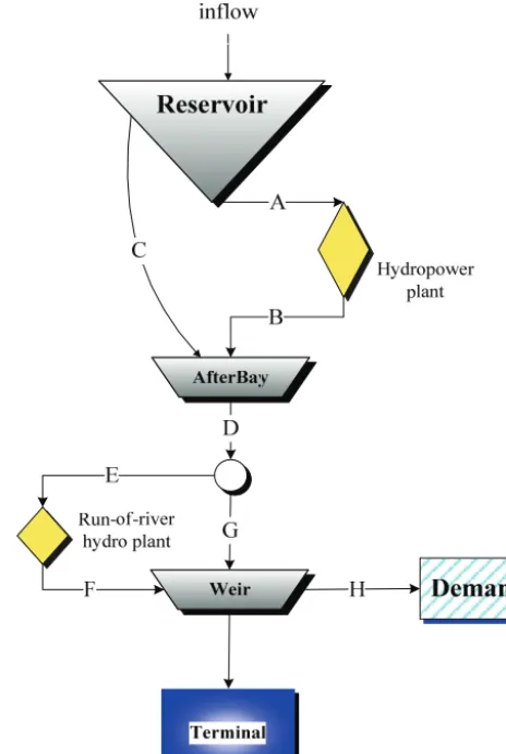
3.3 Rule 3: preferences in water conveyance
Although there are multiple ways to meet a demand, for wa-ter the routes with less transmission loss, lower operating costs, and the potential for additional hydropower genera-tion are generally preferred. This rule allows users to spec-ify the priorities of water conveyance through paths between two specific nodes. For example, possible paths between the reservoir and demand nodes in Fig. 4 are listed in the se-quence of their priorities as follows: (1) A – B – D – E – F – H, (2) A – B – D – G – H, (3) C– D – E – F – H and (4) C – D – G – H.
Suppose that there are np3 possible paths between the
specified source and target nodes. We assume that these paths are arranged in sequence according to their conveyance pri-orities, i.e., if P3k represents thekth path, then water con-veyance throughP3kshould be prior toP3k+1. The function
δ3(i,j )k indicates whetherP3kincludes the link(i, j ). The fol-lowing constraints can then be established:
CMin3k ≤
X (i,j )∈L
δ3(i,j )k c(i,j )≤CMax3k
k=1, ...,np3, (13)
CMax3k+1≤CMin3k+1 k=1, ...,np3−1, (14)
where CMax3k and CMin3k represent the upper and lower
bounds of costs associated with the paths between the speci-fied source and target nodes.
3.4 Rule 4: priorities in multireservoir storage allocation
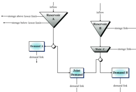
The operation of a multireservoir system involves allocat-ing water from multiple reservoirs to satisfy the joint de-mand. The respective priority rankings for carryover storage of each reservoir determine which reservoir should be used first to satisfy demand throughout a multireservoir system. For example, Fig. 5 depicts a system with two parallel reser-voirs, Reservoirs A and B, both of which can provide wa-ter to the joint demand. Operating rules of this two-reservoir
20
350
Fig. 4 Water supply routes
351
352
3.4
Rule 4: Priorities in multi-reservoir storage allocation
353
The operation of a multi-reservoir system involves allocating water from
354
multiple reservoirs to satisfy the joint demand. The respective priority rankings for
355
carryover storage of each reservoir determine which reservoir should be used first to
356
satisfy demand throughout a multi-reservoir system. For example, Fig.5 depicts a system
357
with two parallel reservoirs, Reservoirs A and B, which both can provide water to the
358
joint demand. Operating rules of this two-reservoir system dictate that joint demand be
359
[image:6.612.312.544.68.414.2]supplied by allocating water from available sources in the following order: (1) first from
360
Figure 4. Water supply routes.
system dictate that joint demand be supplied by allocating water from available sources in the following order: (1) first from Weir C until it has been emptied; (2) then from Reser-voir A, provided that its water level is over its lower limit of rule curve; and (3) finally, from Reservoir B. Accordingly, the storage components can be listed in the sequence of their associated priorities as (1) the storage under the lower limit of Reservoir A, (2) the storage of Reservoir B, (3) the stor-age over the lower limit of Reservoir A and (4) the storstor-age of Weir C.
Assume thatLS(k)represents thekth-priority link in the
set of storage links,LS. The priority constraint for
allocat-ing storage in a multireservoir system can be expressed as follows:
max[cost(RLS(k+1)→JD−RLP)]+
max[cost(RLS(k)−RLP)]< min[cost(RLS(k)→JD−RLP)]+
min[cost(RLS(k+1)−RLP)]k=1, ..., ms−1, (15)
where RLS(k) is the set of all routes with final link as LS(k).RLS(k)→JDconsists of all flow paths that begin at the
F. N.-F. Chou and C.-W. Wu: Priority-based water allocation linear programming model 1863
21
Weir C until it has been emptied; (2) then from Reservoir A, provided that its water level 361
is over its lower limit of rule curve; (3) finally, from Reservoir B. Accordingly, the 362
storage components can be listed in the sequence of their associated priorities as: (1) the 363
storage under the lower limit of Reservoir A, (2) the storage of Reservoir B, (3) the 364
storage over the lower limit of Reservoir A and (4) the storage of Weir C. 365
366
367
Fig. 5 Example of a multi-reservoir system
368
369
Assume that LS(k) represents the kth-priority link in the set of storage links,LS.
370
The priority constraint for allocating storage in a multi-reservoir system can be 371
[image:7.612.49.285.65.224.2]expressed as follows: 372 1 ,...., 1 )] ( cost min[ )] ( cost min[ )] ( cost max[ )] ( cost max[ ) 1 ( ) ( ) ( ) 1 ( − = − + − < − + − + → → + s LP k LP JD k LP k LP JD k m k R R R R R R R R S S S S L L L L (15) 373
Figure 5. Example of a multireservoir system.
reservoir, where the linkLS(k)originates, and culminate by
supplying joint demand.(RLS(k)→JD−RLP)is the same set
after excluding RLP;ms represents the net total of links in LS. The concept of Eq. (15) is explained as follows: suppose
that there is one unit of water initially stored in the reservoir for each of the storage links. The water can either be released to satisfy the joint demand or retained in the reservoir to con-tribute to the associated carryover storage. The left-hand side of Eq. (15) represents the largest cost induced by storing wa-ter in the senior storage link (index k) and releasing water from the junior storage (indexk+1) to supply joint demand. However, the right-hand side represents the lowest cost in-duced by storing and releasing water in the converse way. The inequality ensures that a junior storage will release wa-ter in a higher priority to supply joint demand.
According to similar process as shown from Eq. (4) to Eqs. (7)–(9), the following constraints can be established: CMin4ak ≤
X (i,j )∈L
δ4ak,l(i,j )c(i,j )≤CMax4ak
l=1, ...,np4a,k;k=1, ..., ms, (16)
CMin4bk≤
X (i,j )∈L
δ4b(i,j )k,l c(i,j )≤CMax4bk
l=1, ...,np4b,k; k=1, ..., ms, (17)
CMax4ak+1+CMax4bk+ε≤CMin4ak+CMin4bk+1
k=1, ..., ms−1, (18)
whereCMax4ak andCMin4ak define the feasible range of net
conveyance costs for flow paths represented by(RLS(k)→JD− RLP);CMax4bk andCMin4bk define the feasible range of net
conveyance costs for flow paths represented by (RLS(k)−
RLP); the functionsδ4a(i,j )k,l andδ4bk,l(i,j ) indicate whether the
lth flow path of(RLS(k)→JD−RLP)and(RLS(k)−RLP)
in-clude the link (i, j )respectively; np4a,k and np4b,k are the numbers of paths in(RLS(k)→JD−RLP)and(RLS(k)−RLP)
respectively; andεis the same as in Eqs. (9) and (11).
3.5 Rule 5 (default): minimization of surplus water The proposed method penalizes any water into the final re-ceiving body by the following requirements:
min[cost(RLT)]>0, (19)
max[cost(RLD+LS)]<0, (20)
whereLT is a set that includes all terminal links originated from the node representing the water receiving body;RLT is
a set that consists of all possible flow paths, each of which has a final link that belongs toLT. Equation (19) states that the lowest cost by paths that include the virtual terminal link is greater than zero, and Eq. (20) states the largest cost to a virtual demand or storage link is less than zero. In this man-ner, the NFP algorithm will then try to allocate unregulated flows to water users, and release spill flows from reservoir only if absolutely necessary to prevent inducing a positive cost. The following inequalities can then be established:
X (i,j )∈L
δ5(i,j )k c(i,j )≤ −ε k=1, ...,np5, (21)
X (i,j )∈L
δ6(i,j )k c(i,j )≥ε k=1, ...,np6, (22)
where,δ5(ij )k andδ6(i,j )k are Kronecker delta functions to rep-resent whether link (i,j )is in thekth path inRLD+LS and
RLT, respectively; np5 is the number of paths inRLD+LS;
and np6denotes the number of paths inRLT.
Furthermore, we assume that the cost coefficients of all links other than demand, storage and terminal are greater than 0:
c(i,j )≥0 for all(i, j )∈(L−LD−LS−LT). (23) 3.6 Linear programming for determining cost
coefficients
The constraints, Eqs. (7)–(9), (11)–(12), (13)–(14), (16)–(18) and (21)–(23), define the feasible region for cost coefficients. Linear programming (LP) can be employed to solve the prob-lem, by coupling the constraints with the following objective function:
Minimize X
(i,j )∈(L−LD−LS−LT)
c(i,j ). (24)
1864 F. N.-F. Chou and C.-W. Wu: Priority-based water allocation linear programming model 3.7 Determination of values of the Kronecker delta
functions
The Kronecker delta functions for each link as described in Sects. 3.1–3.5, can be established using the path enumeration algorithm of Kroft (1967). Here a path refers to a sequence of nodes such that from each node there is a link to the next node in the sequence. Furthermore, there should be no cycle, i.e., repetition of nodes, in the path. Repeated identification of possible paths between different associate nodes can help determining the values of the above Kronecker delta func-tions. The computing procedure of Kroft’s algorithm is pro-vided in Appendix A.
4 Case study
The proposed method was applied to determine cost coeffi-cients of the NFP model for simulating the joint water allo-cation of the Hsintein and Tahan rivers’ water resources sys-tem of northern Taiwan. This case study simulates projected conditions of the given system in 2021. The Feitsui Reser-voir, with an effective storage capacity of 336×106m3, is located on Peishih Creek, one of the two major upstream trib-utaries of the Hsintein River. It serves mainly to supply the demand for domestic water in the Taipei (TP) district. Down-stream from the confluence of Peishih and Nanshih Creeks are the Cihukeng, Chihtan, and Chintan weirs, which serve to regulate upstream flow and raise the water level for the diversion of water into three treatment plants. The Cihukeng weir also serves to raise the water level to divert flow into the off-channel Cihukeng hydropower plant through a man-made canal. The tail-water from the hydropower plant is then diverted to the downstream Chintan weir.
The other river in the joint operating system, the Tahan River, has its own reservoir, the Shihmen Reservoir. The ca-pacity of the Shihmen Reservoir is 215×106m3according to the survey in 2011. It was designed for irrigation, hy-dropower generation, public water supply, and flood mod-eration. Downstream from the Shihmen Reservoir are its af-terbay and the Yuanshan weirs, which serve to regulate the reservoir release. The Shanshia pumping station on the Shan-shia River, which is a tributary of the Tahan River, can also support public water supply in this region.
The primary demands for water in the Shihmen Reser-voir system are irrigational and the public demand of south-ern, northern Taoyuan (TY) and Pan-Hsin (PH) districts. The Pingcheng, Longtang, and Shihmen treatment plants with-draw raw water from the Shihmen Reservoir and supply the southern TY district. The northern TY district is supplied by the Danan treatment plant, which withdraws raw water from the Yuanshan weir.
The Tahan River and Hsintien River systems jointly sup-ply the public demand from the PH district. The Panhsin treatment plant receives raw water from both the Yuanshan
27
There is also a trans-basin raw water diversion project being planned in Nanshih 475
Creek in the upstream of Hsintein River, which will focus on building a diversion weir, 476
called Limogan Weir, and a trans-basin tunnel upstream of Nanshih Creek. It aims to 477
divert surplus water from Nanshih Creek to an upper section of Sanshia River, thereby 478
increasing the water utilization efficiency through joint operations. The network of this 479
water resources system is depicted in Fig. 6. 480
Peishih Creek
Nashih Creek
run-of river hydro plant
TaHan River
Shanshia River
Lateral Flow
Limogan Trans-basin tunnel
PH Phase II
Tamsui River
Chihtan
Changhsin
Konkwan
PanHsin DaNan
Shihmen
Longtang Pincheng
TP district PH district
South TY
North TY
Reservoir
Weir
Public Demand
Irrigational Demand
Inflow
Treatment Plant
Hydropower Demand
Environmental Baseflow
Terminal
Hsintein River
Industrial Demand
Taiwan Strait
Cihukeng
Feitsui Reservoir
Chihtan
Chintan Kueishan
Yuanshan AfterBay Shanshia
Weir
Shihmen Reservoir
481
Fig. 6 Joint operation system of Feitsui and Shihmen Reservoirs 482
483
4.1 Priority requirement for trans-basin water diversion 484
The diversion link of Limogan Weir is specified as the last priority link of rule 1, 485
because it should only divert surplus water from Nanshih Creek. This setting ensures 486
Figure 6. Joint operation system of the Feitsui and Shihmen reser-voirs.
weir and Shanshia pumping station. The Hsintien River sys-tem will provide a maximum of 1.01 million m3day−1 of treated water to the PH district after 2016 through the under-construction transbasin pipeline of the “Pan-Hsin Water Sup-ply Improvement Plan, Phase II” (PH-Phase II).
There is also a transbasin raw water diversion project be-ing planned for Nanshih Creek in the upstream of the Hsin-tein River, which will focus on building a diversion weir, called Limogan weir, and a transbasin tunnel upstream of Nanshih Creek. It aims to divert surplus water from Nanshih Creek to an upper section of the Sanshia River, thereby in-creasing the water utilization efficiency through joint opera-tions. The network of this water resources system is depicted in Fig. 6.
4.1 Priority requirement for transbasin water diversion
The diversion link of the Limogan weir is specified as the last priority link of rule 1, because it should only divert sur-plus water from Nanshih Creek. This setting ensures that the transbasin tunnel will not withdraw water originally intended to meet the demands of the Hsintein River system.
4.2 Priority requirement for reservoir operating rule curves
The rule curves of the Feitsui Reservoir include the severe limit (SL), lower limit (LL), middle limit (ML) and upper limit (UL). The Feitsui Reservoir administration specifies the following conditions for operation in 2021 (Chou and Wu, 2011):
1. While reservoir water level is below the SL, it only has to provide 80 % of TP demand.
2. While reservoir level is above the SL but below the LL, it only has to provide 80 % of TP and PH demands.
[image:8.612.311.545.67.238.2]F. N.-F. Chou and C.-W. Wu: Priority-based water allocation linear programming model 1865
29
TP
D80%, (2) SSLF, (3) D80PH%, (4)
F LL S , (5) DTP
%
100 and D100PH%, (6)
F ML
S , (7) F HP P D _ , (8) F
UL S , (9) 507
HP F F
D _ , (10) F FC
S , and (11) SF_W
. 508
TY district TP district
Storage below SL Storage between LL and SL Storage between UL and ML Storage above UL to full capacity
Storage between ML and LL Storage below SL Storage between LL and SL Storage above UL to full capacity
Storage between UL and LL
Shihmen
hydro Peak-hours hydro demand
Peak-hours hydro demand Non-rush-hours hydro demand
Peishih
Creek Tahan River
Nanshih Creek Feitsui hydro Storage 20% demand 80% demand Shanshia River 80% demand 10% demand 10% demand Storage 50% demand 25% demand 25% demand 80% PH 20% PH TP D80%
TP D100%
W F S_
PH D80%
PH D100%
HP F P D_ HP F F D_ F SL S F LL S F ML S F UL S F FC S S SL S S LL S S UL S S FC S TY D80%
TY D90%
TY D100%
A D50%
A D75%
A D100%
W S S_ HP S P D_ Feitsui Reservoir Shihmen Reservoir Weirs Weirs SL: the severe limit of rule curves
LL: the lower limit of rule curves ML: the middle limit of rule curves UL: the upper limit of rule curves
509
Fig. 7 Virtual demand and storage links of the joint operation system of 510
Feitsui and Shihmen Reservoirs 511
512
Shihmen Reservoir operating rule curves must comply with the following criteria: 513
1. While reservoir level is below the SL, it only has to provide 50% of irrigational and 514
80% of TY and PH demands. 515
2. While reservoir level is above the SL but below the LL, it only has to provide 75% of 516
irrigational and 90% of TY demands. 517
Figure 7. Virtual demand and storage links of the joint operation system of the Feitsui and Shihmen reservoirs.
3. While the reservoir level is above the LL, 100 % of the TP and PH demands should be satisfied.
4. While the reservoir level is raised to range between the ML and UL, extra water may be released for peak-hours hydropower generation.
5. Sufficient water should be released to support full-capacity hydropower generation while reservoir level exceeds the UL.
Figure 7, which identifies a variable for each virtual link, illustrates the determination of storage and demand links with respect to the five operating rules delineated above. The codes of virtual links associated with the operating rule curves of the Feitsui Reservoir are listed in the sequence of their associated priorities as follows: (1)D80 %TP , (2)SSLF , (3) D80 %PH , (4)SLLF , (5)D100 %TP andDPH100 %, (6)SMLF , (7)DPF_HP, (8)SULF , (9)DFF_HP, (10)SFCF , and (11)SF_W.
Shihmen Reservoir operating rule curves must comply with the following criteria:
1. While reservoir level is below the SL, it only has to pro-vide 50 % of irrigational and 80 % of TY and PH de-mands.
2. While reservoir level is above the SL but below the LL, it only has to provide 75 % of irrigational and 90 % of TY demands.
3. While the reservoir level is above the LL, 100 % of irri-gational and public demands for the TY district should be satisfied.
4. Extra water should be released to support peak-hour hy-dropower generation while the level is raised beyond the UL.
According to the above operating rules, the setting of virtual storage and demand links of the water resources system of the Tahan River is also depicted in Fig. 7 with a code for each virtual link. The codes of virtual links associated with the operating rule curves of the Shihmen Reservoir are listed in the sequence of their priorities as follows: (1)DA50 %,D80 %TY andD80 %PH , (2)SSLS , (3)D75 %A andDTY90 %, (4)SLLS , (5)DA100 % andD100 %TY , (6)SULS , (7)DS_HPP , (8)SFCS , (9)SS_W, and (10) DPH100 %.
4.3 Priority requirement for the joint operating rules The following rules guide the joint water allocation of this system:
1. The storage of weirs downstream from reservoirs is first allocated to meet demand.
2. While all weirs are dry but the Feitsui Reservoir level exceeds the SL, its storage should be allocated to the PH demand regardless of the Shihmen Reservoir wa-ter level. This means that the priority of Feitsui storage above its SL should be junior than the storage of the Shihmen Reservoir.
3. While all weirs are dry and the Feitsui Reservoir level is unable to attain the SL, water from the Shihmen Reser-voir may be allocated to supply no more than 80 % of the PH demand.
The first condition in the above rules essentially means that the weirs are at the last priority to store water, because their storage is always consumed first. The logic of whether sup-plying water to the joint demand can be used to compare and determine the priorities of different storage components in the Feitsui and Shihmen reservoirs. For instance, water stored in the Feitsui Reservoir under the SL should be se-nior to all Shihmen Reservoir storage, because the third con-dition prevents Feitsui from supplying PH when its storage falls below the SL. Aside from the SL, the priorities of other storage of Feitsui should be junior to the storage of the Shih-men Reservoir, because the Feitsui Reservoir should be the default water source for the PH demand during normal condi-tions. According to these characteristics, the codes of virtual storage links are listed in the order of their associated prior-ities as follows: (1)SSLF , (2)SSLS , (3)SLLS , (4)SULS , (5)SFCS , (6)SLLF , (7)SMLF , (8)SULF , (9)SFCF , (10)SF_WandSS_W. 4.4 Result and discussion
[image:9.612.50.284.67.244.2]1866 F. N.-F. Chou and C.-W. Wu: Priority-based water allocation linear programming model
32
would be -190 (= -270+80), which is larger than the cost of simply storing that water in 560
the storage facilities in the Tahan River system. 561
[image:10.612.51.282.66.214.2]562
Fig. 8 Assigned coefficients based on conditions specified in sections 4.1~4.3 563
564
Assume that both the Feitsui and Shihmen Reservoirs each have one unit of water 565
and that the Feitsui water level is higher than its SL. If the water from Shihmen 566
Reservoir is allocated to supply 80% of the joint demand, the other one unit of water can 567
be stored in Feistui Reservoir to achieve the minimum unit cost of -280. On the other 568
hand, the unit cost of supplying joint demand with Feitsui Reservoir water (and thus 569
retaining Shihmen Reservoir storage) is only -290. Hence, minimum-cost NFP-based 570
water allocation ensures that the joint demand will be satisfied by the Feitsui storage in a 571
higher priority, provided that its water level exceeds the SL. 572
Figure 8. Assigned coefficients based on conditions specified in Sects. 4.1–4.3.
unable to attain the SL. Under these conditions, the alternate supply source, the Shihmen Reservoir, will supply 80 % of the PH district demand. The cost of supplying the remain-ing the PH demand would be−190 (= −270+80), which is larger than the cost of simply storing that water in the storage facilities in the Tahan River system.
Assume that both the Feitsui and Shihmen reservoirs each have one unit of water and that the Feitsui water level is higher than its SL. If the water from the Shihmen Reservoir is allocated to supply 80 % of the joint demand, the other one unit of water can be stored in the Feistui Reservoir to achieve the minimum unit cost of −280. However, the unit cost of supplying joint demand with the Feitsui Reservoir water (and thus retaining the Shihmen Reservoir storage) is only−290. Hence, minimum-cost NFP-based water allocation ensures that the joint demand will be satisfied by the Feitsui storage in a higher priority, provided that its water level exceeds the SL.
The transbasin diversion link in Fig. 8 has a positive cost coefficient of+180. The minimum total cost of paths through this link is−180, which is the sum of the costs of the diver-sion link and the highest priority demand in the Tahan River system. The lowest priority in the Hsintein River system is storage in weirs, each of which has a cost of−210. Thus the model will not allocate water from Nanshih Creek unless all of the weirs of the Hsihtein River are full. In other words, the transbasin tunnel will only divert surplus water from Nanshih Creek.
In the joint operation of Fig. 8, the Feitsui Reservoir is the primary regular source and the Shihmen Reservoir pro-vides the backup source for the PH district. Another oper-ating strategy is to maintain the storage of these two reser-voirs at the same intervals as their individual rule curves. For instance, the storage zones between the LL and SL of both reservoirs would share the same priority. Based on this con-cept of storage balancing joint operation, the virtual storage links are listed in the order of their associated priorities as
34
591
Fig. 9 Cost coefficients for storage balancing of two reservoirs 592
593
Based on Fig. 9, possible joint operating scenarios include the following: 594
1. Any water over the UL in the Shihmen Reservoir will be allocated to the PH district to 595
meet 80% of its full demand, provided that Feitsui level does not exceed its UL. 596
2. When the level of Shihmen Reservoir is between its UL and LL, the Feitsui Reservoir 597
will satisfy the joint demand as long as the its level exceeds the ML. However, if 598
Feitsui storage is unable to attain the LL, then water from the Shihmen Reservoir will 599
be allocated to meet 80% of PH district demand in a higher priority. 600
3. Provided that the Shihmen Reservoir water level ranges between the SL and LL and 601
the water level in the Feitsui Reservoir exceeds the LL, water from Feitsui Reservoir 602
will be allocated to PH district demand. Shihmen Reservoir water will be released to 603
Figure 9. Cost coefficients for storage balancing of two reservoirs.
follows: (1)SSLF , (2)SSLS , (3)SLLF andSLLS , (4)SMLF andSULS , (5) SULF , (6)SFCF and SSFC, (7) SF_W andSS_W. Under this setting, the reservoir with the higher storage is charged with supplying the joint demand to maintain the storage of the two reservoirs in the same interval. The analyzed cost coefficients based on the storage balancing joint operation are illustrated in Fig. 9.
Based on Fig. 9, possible joint operating scenarios include the following:
1. Any water over the UL in the Shihmen Reservoir will be allocated to the PH district to meet 80 % of its full demand, provided that Feitsui level does not exceed its UL.
2. When the level of the Shihmen Reservoir is between its UL and LL, the Feitsui Reservoir will satisfy the joint demand as long as the its level exceeds the ML. How-ever, if Feitsui storage is unable to attain the LL, then water from the Shihmen Reservoir will be allocated to meet 80 % of the PH district demand in a higher priority. 3. Provided that the Shihmen Reservoir water level ranges between the SL and LL and the water level in the Feitsui Reservoir exceeds the LL, water from the Feitsui Reser-voir will be allocated to the PH district demand. Shih-men Reservoir water will be released to independently satisfy 80 % of joint demand only when the Feitsui wa-ter level drops below its SL.
4. When the Shihmen Reservoir water level drops below the SL, the Feitsui Reservoir will independently fulfill the PH district demand provided that its own water level exceeds the SL. If the Feitsui Reservoir water level is below the SL, then the Shihmen Reservoir water will be allocated to ensure that 80 % of the PH demand is satisfied.
In addition to the allocation priorities defined by operating rule curves and joint operating rules, preference for flow
[image:10.612.307.544.68.231.2]F. N.-F. Chou and C.-W. Wu: Priority-based water allocation linear programming model 1867 through a hydropower plant can be simulated by directly
as-signing a negative unit cost to the links connecting to the run-of-river or reservoir hydropower plants to encourage associ-ated flows. Because the interval of costs between consecutive priorities of demands or storage is set as 10, this unit cost will not impair the priority requirements by the above rules, as long as the accumulations of minor costs to demands or reservoirs are within the range between−10 and 10.
5 A pruned analysis procedure
In the aforementioned analysis procedure, the bulk of the computational load is expended on network path enumera-tion analysis. For a complete network, in which every pair of distinct nodes is connected by a unique link (as an extreme example), if there arennodes in the network, then the num-ber of links will be 2×C2n, resulting in
n−2
P i=1
Cin−2paths be-tween any two distinct nodes. This means that the number of paths would grow exponentially with an increase in the num-ber of nodes for such a dense network. The enormous numnum-ber of resulting paths would not only require considerable time for enumeration, but would also expand the size of the subse-quent LP problem. Path enumeration is required because the cost coefficient of every link is assumed to be unknown in the default condition. If additional conditions could be included, such as the assignment of only a few links with nonzero costs and the costs of other links set at 0, then a simpler analysis procedure could be employed to reduce the required compu-tational load.
Using G(N,L) to present the network under analysis, which is defined by a set N of nnodes and a set Lof m links, suppose that there are mP nonvirtual links within L
that are assigned with nonzero costs andmP<m. DefineLP
as the set containing these specified links,NPT andNPHas
the sets of tail and head nodes of links in LP, respectively,
and(ND+NS+NT)as the set that contains all nodes which represent demands, reservoirs or final water receiving bodies inN, and(LD+LS+LT)as the set of demand, storage or terminal links. Then the cost-determining procedure can be simplified as follows:
1. From each of the nodes that convey inflow into the sys-tem, use the depth first search (DFS) algorithm to iden-tify the downstream reachable nodes inG(N,L−LP).
The detail of the DFS algorithm can be found in Ahuja et al. (1993).
2. A fictitious node, denoted as nodef, is created. If node i∈(ND+NS+NT)is identified to be reachable from inflow nodes in the previous step, then a fictitious link (f,i) is created. This fictitious link serves to replace all paths to nodeiwhich consist of only links with zero cost inG(N,L); defineLFas the set that contains these
fictitious links.
3. Use DFS to identify the downstream reachable nodes in
G(N,L−LP)from the head node of each link inLP.
4. Suppose that link (i,j )belongs toLP and nodek
be-longs to eitherNPT or (ND+NS+NT). If k can be reached fromj inG(N,L−LP), then a fictitious link
(j,k)is created and added intoLF. These fictitious links
represent the connectivity between links with nonzero costs.
5. Establish a reduced networkG0(N0,L0)in whichN0is the union ofNPT,NPH,(ND+NS+NT)and nodef, andL0is the union ofL
P,LFand(LD+LS+LT). 6. The same procedure described in Sect. 3 can be
fol-lowed to determine the cost coefficients of links inLP
and(LD+LS+LT), except thatG(N,L)is replaced byG0(N0,L0).
The above procedure takes advantage of the fact that total costs of a path are determined only by the links with nonzero cost coefficients in the path. Thus the enumeration of paths containing all links inLcan be reduced to only enumerating feasible combinations of links inLPand(LD+LS+LT). Be-cause DFS is a basic algorithm with worst-case complexity as onlyO(m), the reduced networkG0can be efficiently
estab-lished from the original networkG. The scale ofG0should be much less thanGbecause typicallymP m. Thus,
enumer-ating paths inG0will require much less computational time and the size of the consequent LP problem can be greatly reduced.
This pruned procedure was employed to finally evaluate the two illustrative problems in Sect. 4. In these final evalua-tions, only the transbasin diversion link and the links con-necting to 20 % joint demand are specified with nonzero costs. The original system was pruned into a reduced network similar to the schematic shown in Fig. 8. For each problem, the number of constraints in the LP formulation was reduced from the original 3227 to only 486. The analysis’ results us-ing the pruned procedure were identical to those as illustrated in Figs. 8 and 9.
6 Conclusions
1868 F. N.-F. Chou and C.-W. Wu: Priority-based water allocation linear programming model treated in a scientific manner in this paper, with systematic
presentations of representative allocation rules encountered in real-world applications. A general procedure is proposed to solve the problem. Although additional analysis efforts are required, the obtained coefficients guarantee that the al-location requirements are satisfied. Thus the possibly time-consuming trial and error process to check the validity of as-signed costs can be avoided.
For an experienced analyst, the adequate assignment of cost coefficients may be done without any preprocessing pro-cedure. But this is not necessarily true for practitioners with less theoretical background, especially when they are deal-ing with systems of complex networks and allocation rules. To a system consists of multiple reservoirs and a transbasin diverting tunnel or pipe as shown in the case study, achiev-ing surplus water diversion and storage allocation inevitably requires assigning nonzero costs on internal links other than demands or storage. This practice is not as straightforward as for systems with simple allocation priorities on demands or reservoir storage. Even for an experienced practitioner, there is always a risk of the wrong assignment of costs due to the variety and complexity of water resources systems. The pro-posed procedure can also serve to validate the effectiveness of the intuitively assigned costs.
Furthermore, if the links to be assigned with nonzero costs can be specified in advance, a simpler procedure can be em-ployed to reduce the computing effort of preprocessing anal-ysis. This procedure prunes the original system into a re-duced network. Thus, the time required to establish and solve the constraints of cost coefficients can be greatly shortened, which further increases the merit of the proposed method.
Acknowledgements. This work was supported by the Water
Re-sources Planning Institute (Grant no. MOEAWRA09600) and the National Science Council (Grant no. NSC 100-2221-E-006-201), Taiwan, R.O.C.
Edited by: G. Characklis
References
Ahuja, R. K., Magnanti, T. L., and Orlin, J. B.: Network Flows: The-ory, Algorithms, and Applications, Prentice-Hall, Upper Saddle River, New Jersey, 1993.
Andreu, J., Capilla, J., and Sanchís, E.: AQUATOOL, a generalized decision support system for water-resources planning and opera-tional management, J. Hydrol., 177, 269–291, 1996.
Andrews, E., Chung, F., and Lund, J.: Multilayer Priority-based simulation of conjunctive facilities, J. Water Res. Pl.-ASCE, 118, 32–53, 1992.
Bessler, F. T., Savic, D. A., and Walters, G. A.: Water reservoir con-trol with data mining, J. Water Res. Pl.-ASCE, 129, 26–34, 2003. Braga, B. and Barbosa, P. F. S.: Multiobjective real-time reservoir operation with network flow algorithm, J. Am. Water Resour. As., 37, 837–852, 2001.
Brendecke, C. M.: Network models of water rights and system op-erations, J. Water Res. Pl.-ASCE, 115, 684–696, 1989.
Cheng, W. C., Hsu, N. S., Cheng, W. M., and Yeh, W. W. G.: A flow path model for regional water distribution optimization, Water Resour. Res., 45, W09411, doi:10.1029/2009WR007826, 2009. Chou, F. N. F. and Wu, C. W.: Reducing the impacts of
flood-induced reservoir turbidity on a regional water supply system, Adv. Water Resour., 33, 146–157, 2010.
Chou, F. N. F., and Wu, C. W.: Assignment of water allocation costs of network flow model, 2011 World Environmental & Water Re-sources Congress, Palm Springs, CA, USA, 22–26 May, 2011. Chung, F. I., Archer, M. C., and DeVries, J. J.: Network flow
algo-rithm applied to California aqueduct simulation, J. Water Resour. Pl.-ASCE, 115, 131–147, 1989.
Dai, T. and Labadie, J. W.: River basin network model for inte-grated water quantity/quality management, J. Water Res. Pl.-ASCE, 127, 295–305, 2001.
Draper, A. J., Munevar, A., Arora, S. K., Reyes, E., Parker, N. L., Chung, F. I., and Peterson, L. E.: CalSim: Generalized model for reservoir system analysis, J. Water Res. Pl.-ASCE, 130, 480– 489, 2004.
Evenson, D. E. and Moseley, J. C.: Simulation/optimization tech-niques for multi-basin water resource planning, Water Resour. Bull., 6 ,725–736, 1970.
Ferreira, I. C. L.: Deriving unit cost coefficients for linear programming-driven priority-based simulations, Ph.D. disserta-tion, University of California Davis, USA., 133 pp., 2007. Fredericks, J. W., Labadie, J. W., and Altenhofen, J. M.: Decision
support system for conjunctive stream-aquifer management, J. Water Resour. Pl.-ASCE, 124, 69–78, 1998.
Gandolfi, C., Guariso, G., and Togni, D.: Optimal flow allocation in the Zambezi River system, Water Resour. Manage., 11, 377–393, 1997.
Hydrologics, Inc.: User manual for OASIS with OCLTM, Columbia, Maryland, USA, 2009.
Ilich, N.: Shortcomings of linear programming in optimiz-ing river basin allocation, Water Resour. Res., 44, W02426, doi:10.1029/2007WR006192, 2008.
Ilich, N.: Limitations of network flow algorithms in river basin mod-eling, J. Water Resour. Pl.-ASCE, 135, 48–55, 2009.
Ilich, N., Simonovic, S. P., and Amron, M.: The benefits of comput-erized real-time river basin management in the Malahayu Reser-voir System, Can. J. Civil Eng., 27, 55–64, 2000.
Israel, M. and Lund, J.: Priority preserving unit penalties in network flow modeling, J. Water Res. Pl.-ASCE, 125, 205–214, 1999. Juízo, D. and Lidén, R.: Modeling for transboundary water
re-sources planning and allocation: the case of Southern Africa, Hydrol. Earth Syst. Sci., 14, 2343–2354, doi:10.5194/hess-14-2343-2010, 2010.
Khaliquzzaman and Chander, S.: Network flow programming model for multireservoir sizing, J. Water Res. Pl.-ASCE, 123, 15–22, 1997.
Kroft, D.: All paths through a maze, P. IEEE, 55, 88–90, 1967. Kuczera, G.: Fast multireservoir multiperiod linear programming
models, Water Resour. Res., 25, 169–176, 1989.
Kuczera, G. and Diment, G.: General water supply system simula-tion model: WASP, J. Water Res. Pl.-ASCE, 114, 365–382, 1988.
F. N.-F. Chou and C.-W. Wu: Priority-based water allocation linear programming model 1869
Labadie, J. W.: Optimal operation of multireservoir systems: A state-of-the-art review, J. Water Res. Pl.-ASCE, 130, 93–111, 2004.
Labadie, J. W. and Baldo, M.: Discussion of: “Priority preserving unit penalties in network flow modeling”, by Israel, M. and Lund, J., J. Water Res. Pl.-ASCE, 125, 67–68, 2001.
Labadie, J. W., Bode, D. A., and Pineda, A. M.: Network model for decision-support in municipal raw water supply, Water Resour. Bull., 22, 927–940, 1986.
Lund, J. R. and Ferreira, I.: Operating Rule Optimization for Mis-souri River reservoir system, J. Water Res. Pl.-ASCE, 122, 287– 295, 1996.
Martin, Q. W.: Hierarchical algorithm for water supply expansion, J. Water Res. Pl.-ASCE, 113, 677–695, 1987.
Rani, D. and Moreira, M. M.: Simulation–optimization modeling: a survey and potential application in reservoir systems operation, Water Resour. Manage., 24, 1107–1138, 2010.
Sigvaldason, O. T.: A simulation model for operating a multipur-pose multireservoir system, Water Resour. Res., 12, 263–278, 1976.
Stockholm Environment Institute: WEAP: Water evaluation and planning system-user guide, Boston, USA, 2011.
Wurbs, R.: Reservoir system simulation and optimization models, J. Water Res. Pl.-ASCE, 119, 455–471, 1993.
1870 F. N.-F. Chou and C.-W. Wu: Priority-based water allocation linear programming model Appendix A: Kroft’s path enumeration algorithm
Kroft’s algorithm aims to find all paths that connect a source nodesand a target nodet. It uses a stack (a data structure that stores elements in a last in, first out manner) to store the path that has been built by the algorithm thus far. The recursive procedure is as follows:
1. Upon entering the procedure, the element at the top of the stack, say node i, is selected. The procedure searches for the first outgoing link of nodei, say link (i,j )of which the head node (nodej )is not already on the stack.
2. If a nodej is found, then it is added to the stack. a. Ifj=t, then the elements in the stack represent a
new path froms tot. The path is output and j is deleted from the stack.
b. If j 6=t, then the above steps are repeated recur-sively.
3. If the algorithm is unable to find a link (i,j )for which nodejis not already on the stack, nodeiis deleted from the stack. The above steps are then repeated recursively. When the above procedure is called for the first time, only source node s is initially contained within the stack in the algorithm. The algorithm terminates when the stack is empty. While implementing Kroft’s algorithm, a number of pro-gramming techniques similar to a common DFS algorithm are also used. For instance, an adjacency list may be used to store the network structure. The adjacency list for node i, denoted asA(i), is defined as the set of links emanating from nodei. A data structure comprising a singly linked list is used to establish an adjacency list for every node in the network. An array of pointer variables, known as first (i), is used to point to the first link ofA(i)for eachithat belongs to
N. Another pointer array, current arc (i), is also used to store the next candidate link that the algorithm is going to exam-ine from nodei. More details related to these skills and their implementation for a DFS algorithm can be found in Ahuja et al. (1993).
F. N.-F. Chou and C.-W. Wu: Priority-based water allocation linear programming model 1871 Appendix B: A simplified demonstration example
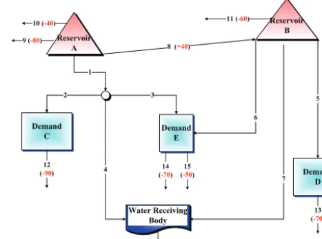
Figure B1 depicts the network of an example simplified from the case study to demonstrate the LP formulation established by the proposed method. In this example, a specific index number designates each respective link. The carryover stor-age of Reservoir A is represented by two dotted virtual links, numbers 9 and 10, which represent the capacities below and above the rule curve, respectively. Two virtual links, num-bers 14 and 15, are assigned to Demand E to represent 80 % and 20 % of its total demand, respectively. The parenthesized numbers for link number 8 and all virtual links represent the assigned nonzero cost coefficients derived from the rules shown from B.1 to B.4:
B1 Priority requirement for reservoir operating rule curves
The assumed allocation priorities of Reservoir A and its ac-cessible downstream demands are as follows: (1) satisfying Demand C, (2) elevating storage of Reservoir A up to its rule curve, (3) satisfying Demand E and (4) filling Reservoir A. According to Eqs. (11) and (12), the established inequalities will be
CAMin21≤c1+c2+c12≤CAMax21, (B1)
CAMin22≤c9≤CAMax22, (B2)
CAMin23≤c1+c3+c14≤CAMax23, (B3)
CAMin24≤c1+c3+c15≤CAMax24, (B4)
CAMin25≤c10≤CAMax25, (B5)
CAMax2k+ε≤CAMin2k+1 fork=1−4, (B6)
wherecirepresents the cost coefficient of link numberi. The assumed allocation priorities of Reservoir B and the associ-ated demands are (1) satisfying Demand D and 80 % of De-mand E, (2) storing all surplus water in Reservoir B and (3) fulfilling Demand E. Consequently, the established inequali-ties are
CBMin21≤c5+c13≤CBMax21, (B7)
CBMin21≤c6+c14≤CBMax21, (B8)
CBMin22≤c11≤CBMax22, (B9)
CBMin23≤c6+c15≤CBMax23, (B10)
CBMax2k+ε≤CBMin2k+1 fork=1−2. (B11)
B2 Priority requirement for the joint operating rules According to Eqs. (16)–(18), if the priorities of storage al-location are (1) the capacity below rule curve of Reservoir A, (2) the total storage of Reservoir B and (3) the capacity above the rule curve of Reservoir A, the converted constraints
42
Demand E Demand
C
Demand D
1
3
6
5 2
Reservoir B Reservoir
A 8 (+40)
Water Receiving Body
4
7 10 (-40)
9 (-80)
11 (-60)
12 (-90)
13 (-70) 14
(-70) 15 (-50)
16 (+10)
747
Fig. 10 Network of a simplified example
748
749
B.1. Priority requirement for reservoir operating rule curves
750
The assumed allocation priorities of Reservoir A and its accessible downstream
751
demands are as follows: (1) satisfying Demand C, (2) elevating storage of Reservoir A
752
up to its rule curve, (3) satisfying Demand E and (4) filling Reservoir A. According to
753
Eqs. (11) and (12), the established inequalities will be:
754
1
1 1 2 12 2
2 Max
Min c c c CA
CA ≤ + + ≤
(25)
755
2
2 9 2
2 Max
Min c CA
CA ≤ ≤
(26)
756
3
3 1 3 14 2
2 Max
Min c c c CA
CA ≤ + + ≤
(27)
757
Figure B1. Network of a simplified example.
would then be
CMin4b1 ≤c9≤CMax4b1, (B12)
CMin4b2 ≤c11≤CMax4b2, (B13)
CMin4b3 ≤c10≤CMax4b3, (B14)
CMin4a1≤c1+c3≤CMax4a1, (B15)
CMin4a2≤c6≤CMax4a2, (B16)
CMax4a2+CMax4b1+ε≤CMin4a1+CMin4b2, (B17)
CMax4a1+CMax4b2+ε≤CMin4a2+CMin4b3. (B18)
B3 Priority requirement for transbasin water diversion
Link number 8 is specified as the last priority link, which will produce the following constraints according to Eqs. (7)–(9):
c8+c11≥CMin1, (B19)
c8+c5+c13≥CMin1, (B20)
c8+c6+c14≥CMin1, (B21)
c8+c6+c15≥CMin1, (B22)
CAMax25+ε≤CMin1, (B23)
CBMax23+ε≤CMin1. (B24)
B4 Linear programming formulation
In addition to the above rules, the net costs of paths into the terminal water receiving body are designed to be positive:
c1+c4+c16≥ε, (B25)
c8+c1+c4+c16≥ε, (B26)
c7+c16≥ε. (B27)